Notes on Computational Fluid Dynamics: General Principles

Chapter 2 Fluid Dynamics

This chapter introduces fluid dynamics for CFD. It describes: governing equations, i.e. conservation of mass, momentum and energy; and, associated physical models, e.g. for viscosity, heat conduction and thermodynamics.

The equations describe fluid motion, forces and heat in time and three-dimensional (3D) space. Vector notation provides a mathematical framework to present the equations in a compact form. It enables the equations to be presented independently of any co-ordinate system, e.g. Cartesian (//) or spherical (//). It includes a standard set of algebraic operations, e.g. the inner (dot) and outer products.

The notation helps to ensure that the terms in equations are unchanged, or invariant, under a co-ordinate system transformation. Without invariance, a flow solution, e.g. along a pipe, would be dependent on the orientation of the pipe with respect to the co-ordinate system. Logically this dependence cannot exist; the laws of motion are the same in all “inertial frames”.¹

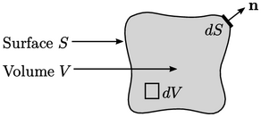
The derivation of the governing equations uses a control volume bounded by a surface , presented using the two-dimensional (2D) illustration above. We use and to describe an infinitesimally small volume and surface, respectively, and is the unit normal vector for each increment of surface , discussed in Sec. 2.1 . It is important to note in any derivation whether the volume is defined as fixed in space or moving with the fluid.

Each derivation generally begins with a definite integral of some quantity, e.g. , over the volume denoted by

(2.1)

If this notation is unfamiliar, understand it to mean a summation for all increments of volume that make up the total volume . The summed values are , where is the value in the respective .

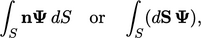
The derivations also use integrals over the surface , e.g.

(2.2)

where . Volume and surface integrals are connected through Gauss’s Theorem, introduced in Sec. 2.4 .

---

---