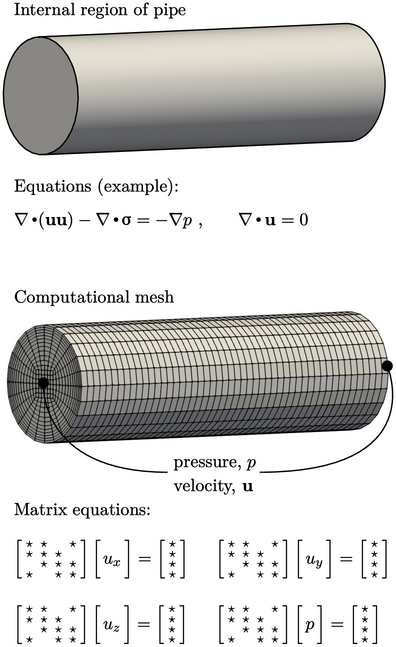
1.1 Solution overview
Let us imagine calculating fluid flow along a pipe with CFD. To perform the calculation first requires a description of the problem by:
- the domain occupied by the fluid, i.e. the internal region of the pipe;
- equations that represent the fluid behaviour, in
terms of properties such as pressure
 and velocity
 ;
; - conditions at the boundary of the fluid domain and initially within the domain for the fluid properties.
This description is represented in CFD by the following:
- a computational mesh for the fluid;
- “discrete” equations and algorithms to
calculate
 and
and  ;
; - boundary and initial conditions for
 and
and
 .
.
Chapter 2 introduces the governing equations and basic models for fluid motion, forces and heat. Turbulence, which commonly occurs in many flows, is introduced in Chapter 6 and its standard modelling is described in Chapter 7 .
The finite volume method is presented in Chapter 3 to express equations in discrete form using its geometric representation of a computational mesh. The algorithms used to solve the matrix equations and to couple sets of equations are given in Chapter 5 .
Chapter 4 describes boundary conditions first from a numerical perspective, i.e. how they modify the matrix equations to influence the solution. It then covers a range of conditions that represent the behaviour at boundaries in many problems.