
2.13 Incompressible flow
We can derive a set of equations for incompressible flow that includes:
- mass conservation, Eq. (2.8 );
- momentum conservation, Eq. (2.19 );
- the material derivative for
 , Eq. (2.26
);
, Eq. (2.26
); - the rate of deformation tensor, Eq. (2.33 );
- the Newtonian fluid model, Eq. (2.41 ).
Combining Eq. (2.41 ) and Eq. (2.33 ) and using Eq. (2.36 ) for the deviatoric part of a tensor, gives an expression for stress:
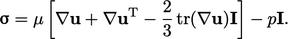 |
(2.44) |
 into Eq. (2.19
) and applying
Eq. (2.26
) gives an equation
for momentum for a Newtonian fluid:
into Eq. (2.19
) and applying
Eq. (2.26
) gives an equation
for momentum for a Newtonian fluid:
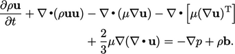 |
(2.45) |
 on
page 84
.
on
page 84
.
An incompressible fluid exhibits  constant over
time, i.e. for moving volumes of fluid
constant over
time, i.e. for moving volumes of fluid  Combining the
material derivative Eq. (2.14
) and mass
conservation Eq. (2.8
) gives
Combining the
material derivative Eq. (2.14
) and mass
conservation Eq. (2.8
) gives 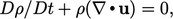 which results in the
incompressibility
condition
which results in the
incompressibility
condition
 |
(2.46) |
A homogeneous, incompressible material
exhibits  = constant uniformly throughout the entire fluid. With that assumption,
Eq. (2.45
) can be written as
= constant uniformly throughout the entire fluid. With that assumption,
Eq. (2.45
) can be written as
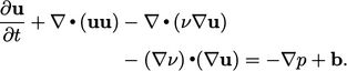 |
(2.47) |
 in SI units of
 ;
and
;
and  represents kinematic
pressure, i.e. divided by
represents kinematic
pressure, i.e. divided by  , in SI units of
 .
.
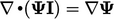
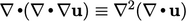
The identity  and the
incompressibility Eq. (2.46
) yield the terms in
Eq. (2.47
).
and the
incompressibility Eq. (2.46
) yield the terms in
Eq. (2.47
).
Pressure equation
Mass and momentum conservation, represented by
Eq. (2.46
) and
Eq. (2.47
) respectively,
provide two equations — one scalar, one vector — for two fields,
 and
and
 .
However, Eq. (2.46
) cannot be solved in
its own right since it provides only one equation for vector
.
However, Eq. (2.46
) cannot be solved in
its own right since it provides only one equation for vector
 ,
containing 3 components.
,
containing 3 components.
A scalar equation, including both  and
and  , can be derived by
taking the divergence of
Eq. (2.47
) and eliminating
terms by substituting Eq. (2.46
), noting that
, can be derived by
taking the divergence of
Eq. (2.47
) and eliminating
terms by substituting Eq. (2.46
), noting that
 .
For
.
For  and
and  that are constant and uniform, the equation is
![2 r p + r [r (uu)] = 0: \relax \special {t4ht=](img/index614x.png) |
(2.48) |
 and
and
 .
Chapter 5
describes the algorithms
used in the finite volume method which couple the two equations
using a modified form of Eq. (2.48
).
.
Chapter 5
describes the algorithms
used in the finite volume method which couple the two equations
using a modified form of Eq. (2.48
).
