Notes on Computational Fluid Dynamics: General Principles

Chapter 4 Boundary Conditions

Chapter 3 described:

• the computational mesh consisting of cells of any irregular polyhedral shape with mesh properties for the finite volume method;
• discretisation of terms in equations to construct a matrix equation for solution variable ;
• discretisation schemes for optimal accuracy, boundedness and convergence, using limiting and correction;
• the time derivative, Courant number and time step size.

At the boundary of the mesh, constraints must be applied to the solution variable , known as boundary conditions. Setting boundary conditions is challenging because:

• they need to reflect the physical conditions of the case being simulated;
• they need to make the case well posed, i.e. provide unique, stable, physical solutions to the equations;
• they must be compatible across sets of multiple equations, in particular and .

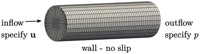
The mesh boundary is split into regions known as patches, on which different boundary conditions are applied. The choice of boundary condition generally depends on flow direction at a patch, whether the patch corresponds to a solid wall, etc.

There are basic forms of boundary condition which specify the value, normal gradient, etc. of at the boundary. They are applied through modifications to the matrix coefficients and source vector using mesh data of the faces and cells adjacent to the boundary.

The opening topics of this chapter describe the mesh data and the numerical methods required by the basic forms of boundary condition.

More specialised boundary conditions can be derived from the underlying forms which correspond to different physical conditions. Some derived conditions, that are often used for particular boundary configurations, are introduced in this chapter.

Otherwise, the number of possible derived conditions is almost unlimited due to the range of potential physical conditions that can be encountered in fluid flow problems. It is left to the producers of CFD software to document those conditions, when it is important that the user identifies the basic underlying type of the condition, e.g. fixed value or gradient.