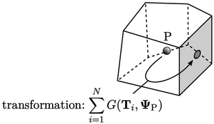
4.11 Transform condition
Some boundary conditions represent  at the
boundary as a transformation of the cell value
at the
boundary as a transformation of the cell value  . They can be expressed
in terms of a general transform condition
. They can be expressed
in terms of a general transform condition
|
(4.13) |
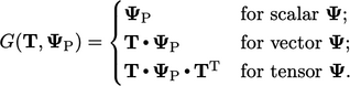
where

is the geometric transformation of variable

by a tensor

.
The transformation is calculated
as follows:
|
(4.14) |
When

is a scalar, the transform condition is equivalent to a
zero gradient condition. Otherwise, it is implemented so that terms
in

in Eq. (
4.13
) contribute to coefficients in

.
These contributions are implicit which improves convergence when
solving the matrix equation
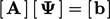
.
A factor  is introduced to specify the contribution
to internal coefficients. It represents a single internal coefficient
for each component of
is introduced to specify the contribution
to internal coefficients. It represents a single internal coefficient
for each component of  so has the same rank
as
so has the same rank
as  , i.e. it is a
vector when
, i.e. it is a
vector when  is a vector, and a tensor when
  is a tensor.
The multiplication of each coefficient of
 by
its respective component of
by
its respective component of  is denoted by by
 .
In the case of vector
.
In the case of vector  , this “component multiplication” is
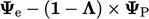
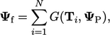
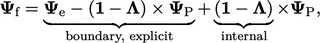
For advection discretisation, the face value is represented as
|
(4.15) |
where

is an explicit boundary value,
calculated from the expression in
Eq. (
4.13
) using the current values

.
The other explicit term uses the current

with “

” denoting

for a vector

and

for a tensor.
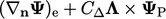
Laplacian discretisation requires the face normal
gradient  . Combining
 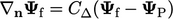 with Eq. (4.15
) gives
with Eq. (4.15
) gives
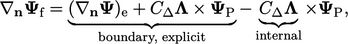
|
(4.16) |
where the explicit gradient is calculated by

|
(4.17) |
The transform condition is summarised within the table below by the
value and gradient contributions.