Notes on Computational Fluid Dynamics: General Principles

[chapter contents][previous topic][next topic][index]

4.9 Mixed ﬁxed value/gradient

Sec. 4.8 concluded with a table of factors for the contributions to coeﬃcients of $\text{[math]}$ and $\text{[math]}$ for the ﬁxed value and ﬁxed gradient boundary conditions.

It distinguishes between contributions for the discretisation of an advection term which requires values at faces, and the Laplacian term which requires the normal gradient.

A mixed ﬁxed value/gradient condition is deﬁned by introducing a value fraction $\text{[math]}$ for which

(0 represents ﬁxed gradient, v = 1 represents ﬁxed value. \relax \special {t4ht=

(4.9)

Within the range $\text{[math]}$ the condition operates in between ﬁxed value and ﬁxed gradient. The mixed condition is simply implemented by blending the ﬁxed value and ﬁxed gradient contributions by $\text{[math]}$ , as shown in the table below.

factor	mixed

value internal	$\text{[math]}$
value boundary	$\text{[math]}$
gradient internal	$\text{[math]}$
gradient boundary	$\text{[math]}$

This mixed condition provides the framework for a boundary condition that can switch between a ﬁxed value $\text{[math]}$ and ﬁxed gradient $\text{[math]}$ , by changing $\text{[math]}$ . Switching is often based on ﬂow direction, $\text{[math]}$ corresponding to inﬂow and $\text{[math]}$ to outﬂow.

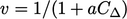
Some boundary conditions can operate in the range of value fractions $\text{[math]}$ . The Robin condition, described next, can also be expressed as a mixed condition with varying $\text{[math]}$ .

Robin condition

The Robin condition⁵ combines the value and normal gradient at the boundary through an expression:

+ arn = 0; \relax \special {t4ht=

(4.10)

where $\text{[math]}$ is a scalar coeﬃcient with units of length and $\text{[math]}$ is some constant value of $\text{[math]}$ .

The Robin condition can be treated like the mixed condition by relating $\text{[math]}$ to a reference ﬁxed value $\text{[math]}$ and gradient $\text{[math]}$ at a boundary, according to $\text{[math]}$ .

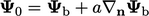Substituting for $\text{[math]}$ in Eq. (4.10) and making $\text{[math]}$ the subject of the equation gives:

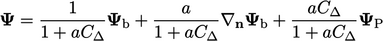= ---1---- b +----a---rn b + -aC----- P 1+ aC 1 + aC 1+ aC \relax \special {t4ht=

Comparison with the value factors in the previous table shows that the Robin condition corresponds to the mixed condition with the value fraction $\text{[math]}$ .

In this form, $\text{[math]}$ and $\text{[math]}$ relate to the limits $\text{[math]}$ and $\text{[math]}$ , respectively. Values can be selected in these limits to represent the physics of the condition.

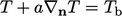In many cases the reference gradient is $\text{[math]}$ such that $\text{[math]}$ in Eq. (4.10 ). For example a condition for temperature $\text{[math]}$ would tend to $\text{[math]}$ as $\text{[math]}$ and $\text{[math]}$ as $\text{[math]}$ .

The value fraction $\text{[math]}$ includes $\text{[math]}$ , so the condition operates “in the middle” between the ﬁxed value and gradient when $\text{[math]}$ is the same order of magnitude as the boundary cell height.

⁵after Victor Robin (1855-1897).

Notes on CFD: General Principles - 4.9 Mixed ﬁxed value/gradient