
4.12 Symmetry condition
The transform boundary condition was presented in Sec. 4.11 . It provides a convenient framework for implementing boundary conditions that represent a geometric constraint, including the symmetry condition.
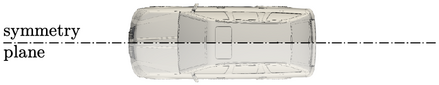
The symmetry condition is suitable for simulations where the geometry contains a plane of symmetry and the flow field is assumed symmetric. By generating a mesh on one side of a plane of symmetry and applying the symmetry condition, the number of cells, and hence solution time, is reduced.
In the context of a wall boundary, the symmetry condition is also equivalent to slip (as opposed to the common no-slip condition).
A symmetry plane is a transform condition so when
the solution variable  is a scalar, it reduces to zero gradient. For a
vector, e.g.
is a scalar, it reduces to zero gradient. For a
vector, e.g.  , the condition
is zero gradient tangential to the plane, and zero fixed value
normal to the plane.
, the condition
is zero gradient tangential to the plane, and zero fixed value
normal to the plane.
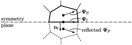
When  is a tensor, the boundary condition
requires a more precise definition, which can also be applied to a
vector
is a tensor, the boundary condition
requires a more precise definition, which can also be applied to a
vector  . The boundary
  can be considered as the mean of the adjacent
cell
can be considered as the mean of the adjacent
cell  and the mirror image
  transformed by the
reflective transformation tensor
transformed by the
reflective transformation tensor  , i.e.
![1 f = 2-[ P + G(I 2nfnf; P)]: \relax \special {t4ht=](img/index1828x.png) |
(4.18) |
 is the unit normal vector on the boundary face.
Using the notation in Sec. 4.11
, the explicit boundary
value  is calculated using current
  from
Eq. (4.18
) and the explicit
gradient
from
Eq. (4.18
) and the explicit
gradient  is calculated by Eq. (4.17
).
is calculated by Eq. (4.17
).
Comparing Eq. (4.18)
with the transform condition of Sec. 4.11
, the factor  corresponds to the
tensor
corresponds to the
tensor  . For a vector field, a factor which gives good solution
convergence is
. For a vector field, a factor which gives good solution
convergence is
 |
(4.19) |
 ” is the vector of the diagonal components of tensor
 .
.
For a tensor field, good convergence is achieved
with a tensor  calculated as the outer product of
  for a vector,
i.e. denoting the vector
factor by
for a vector,
i.e. denoting the vector
factor by  , the tensor factor is
 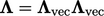 .
.
Orthogonality condition
The axes  ,
,  ,
,  , introduced in
Sec. 2.1
, must remain orthogonal under
a transformation. It requires the transpose of the transformation
tensor
, introduced in
Sec. 2.1
, must remain orthogonal under
a transformation. It requires the transpose of the transformation
tensor  to equal its inverse, i.e.
  .
.
The orthogonality condition is therefore
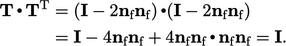
 The reflective transformation
 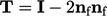 satisfies the
orthogonality condition since
satisfies the
orthogonality condition since
 |
