Notes on Computational Fluid Dynamics: General Principles

4.1 Boundary mesh

Sec. 3.2 describes the computational mesh used by the finite volume method. It identifies a domain boundary by faces which are connected only to one cell. The boundary faces are grouped into patches, each under a unique name, corresponding to different regions of the boundary. Boundary conditions are then applied to each patch to provide a representative solution to the case of interest.

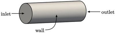
In the example of flow in a pipe, it would be logical to split the boundary into 3 patches in order to specify inflow, outflow and solid walls; and, inlet, outlet and wall would be logical names for these patches.

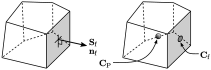
Patch geometric data

The geometry of a patch is described using face data described in Sec. 3.3 , including:

• the face area vector , with area magnitude and direction ;
• the face unit normal vector ;
• the face centre .

The cell connected to each patch face is denoted by the subscript “P”, e.g. the cell centre is denoted .

Patch deltas

Sec. 3.8 describes the “delta” for each face as the vector connecting the centres of its owner and neighbour cells. is defined differently for a patch face since it has no neighbour cell.

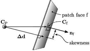
The delta is defined as the component of in the face normal direction. The surface gradient is orthogonal to the face, which eliminates the error associated with non-orthogonality, at the expense of introducing a skewness error. Taking the inner product with gives the magnitude which is then multiplied by to assign the direction, i.e.

(4.1)

The delta coefficients are , as defined in Sec. 3.8 . The delta coefficient , representing “inverse distance”, is a critical parameter in the discretisation of boundary conditions.