Notes on Computational Fluid Dynamics: General Principles

4.10 Mixed inlet-outlet condition

The inlet-outlet boundary condition is the most basic example of the mixed fixed value/gradient type, described in Sec. 4.9 . The condition sets the reference gradient and uses a specified reference value . The value fraction is then set to

(4.11)

The flow direction is established from the sign of the volumetric or mass flux at each boundary face, described in Sec. 2.8 , by

(4.12)

The inlet-outlet condition is generally very useful for scalar fields, e.g. turbulence fields, , etc. It has an immediate practical use at a free boundary, e.g. in the case introduced in Sec. 4.6 .

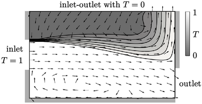
The figure shows the solution of Eq. (2.65 ), converged over time with and unity Prandtl number , see Sec. 2.21 . The fixed condition is applied at the inlet and a zero gradient condition at the walls.

At the free boundary, the inlet-outlet condition enables to be specified where inflow occurs. The inlet value in the example is set to ; the image shows mixing of fluids at different temperatures, from the inlet and entrained at the free boundary.

Numerical benefit of inlet-outlet

Boundaries may be described “inlet” and “outlet” based on the expectation of the flow direction during a simulation. But the flow direction may not always happen as expected.

In the case of an outlet, for example, inflow might occur during a simulation. For example, at the start of a simulation, the initial conditions may induce inflow before the internal flow is established. Localised inflow can also occur when rotating flow structures pass through an outlet boundary, e.g. when a bluff body sheds vortices, as shown below.

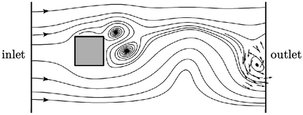
Where inflow occurs, the inlet-outlet condition can switch to the fixed value type to ensure stability, as discussed in Sec. 4.5 . The inlet-outlet condition is therefore commonly applied to scalar fields (except ), at a boundary which is notionally an outlet, to avoid numerical instability associated with unexpected inflow.