Notes on Computational Fluid Dynamics: General Principles

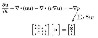
3.24 Example of building a matrix equation

The previous sections describe methods to discretise derivative and other terms in order to build a matrix equation for a given physical equation. Let us demonstrate the construction of a matrix equation, using the momentum conservation equation from Sec. 3.23 as an example. It is a vector equation, so produces 3 matrix equations for , and .

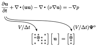
The first term, the time derivative , might be discretised with the Euler scheme Eq. (3.21 ). Matrix equations are constructed in extensive form as discussed in Sec. 3.6 . Hence, the contributions from Eq. (3.21 ) to matrix coefficients and source vector are scaled by cell volume , i.e. and , respectively, as illustrated below.

The second term, the advective derivative , is discretised by Eq. (3.8 ). It pre-calculates the volumetric flux , using interpolated by Eq. (3.3 ) with linear weights Eq. (3.4 ).

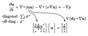
The transported might be discretised using the linear upwind scheme described in Sec. 3.14 . The scheme first applies upwind discretisation, which contributes outgoing positive fluxes to diagonal coefficients and negative fluxes to off-diagonals. It then adds an explicit contribution based on an extrapolated gradient (see Sec. 3.14 ). The gradient is usually calculated by Eq. (3.18 ) with gradient limiting from Sec. 3.16 .

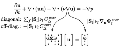
The third term, the Laplacian derivative , is discretised by Eq. (3.2 ). It requires , which is linearly interpolated from the cell centres. If the surface normal gradient includes a non-orthogonal correction , see Sec. 3.8 , then the term contributes to and , as shown below.

The final term, is calculated using Eq. (3.18 ). Like all the other terms described here, it is implemented in extensive form, scaling by , so is calculated for each cell by the vector . The relevant component (, , ) of this vector is then applied to the respective equation for , and .