Notes on Computational Fluid Dynamics: General Principles

4.13 Axisymmetric (wedge) condition

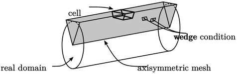
There are some fluid flow problems for which the geometry is axisymmetric. Assuming the flow solution is axisymmetric, i.e. fields do not change in the circumferential direction, the computational mesh can be formed of a wedge-shaped slice of the flow geometry.

This type of mesh for axisymmetric solution contains one cell across the circumferential direction, which reduces the number of cells to two dimensions in the axial and radial directions.

This approach to axisymmetric solution introduces a geometric error due the faces normal to the radial direction being flat. This error reduces with decreasing wedge angle; in practice, the error can be considered negligible for an angle of 1.

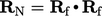
The wedge boundary condition is applied to the two sloping side patches. It transforms cell values to the patch faces using a rotational transformation tensor by

(4.20)

defines a rotation between the unit vector in the circumferential direction at the cell centre and the unit face normal vector by

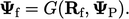
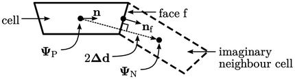
The wedge condition uses the general transform framework of Sec. 4.11 , with the explicit value calculated using current from Eq. (4.20). The explicit gradient is the boundary gradient calculated from in an imaginary neighbour cell by

(4.21)

where the rotation between cell centres .

The factor is chosen to minimise the gradient boundary coefficients (see Sec. 4.11 ). The vector factor is where “” is defined in Sec. 4.12 .

For a tensor , the factor is , where are the coefficients for a vector, as described for the symmetry condition in Sec. 4.12 .

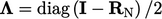
Rotation tensor

The rotation tensor between two unit vectors and can be calculated using the Euler-Rodrigues rotation formula,⁶

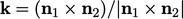where and .

---

---