
4.8 Numerical framework
The fixed value and fixed gradient conditions described in Sec. 4.2 can be combined to form a general numerical framework for boundary conditions.
The contributions from the boundary conditions to
the matrix equation 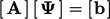 , by discretisation of advection and Laplacian
terms, can be generalised as:
, by discretisation of advection and Laplacian
terms, can be generalised as:
- “internal” contributions to
 , from terms
including the cell value
, from terms
including the cell value  ;
; - “boundary” contributions to
 , from terms
without
, from terms
without  .
.
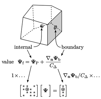
The example above shows Eq. (4.2
) for the face
value, required at a boundary for advection discretisation, in the
case of a fixed gradient
boundary condition. The internal “factor” on  is 1, which is
multiplied by
is 1, which is
multiplied by  for the contribution to the respective diagonal
coefficient in
for the contribution to the respective diagonal
coefficient in  , as in the example in Sec. 3.24
.
, as in the example in Sec. 3.24
.
The boundary factor is  , which is similarly
multiplied by
, which is similarly
multiplied by  for the contribution to
  .
.
For the fixed
value condition  with advection, the boundary factor is
 and an internal factor is 0.
Laplacian discretisation requires the surface
normal gradient on the faces. A fixed gradient condition delivers an
equivalent boundary factor of  to
to  and an internal
factor of 0.
and an internal
factor of 0.
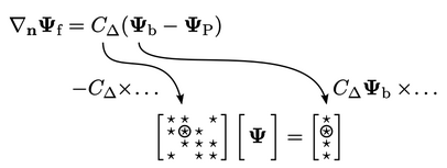
 ,
the face normal gradient Eq. (4.3
) gives an internal
factor of
,
the face normal gradient Eq. (4.3
) gives an internal
factor of  and a boundary factor of
  . Both are multiplied
by
. Both are multiplied
by  in their contributions to
  and the diagonal coefficient of
  in
in
 ,
as shown in the Laplacian discretisation in Sec. 3.24
.
,
as shown in the Laplacian discretisation in Sec. 3.24
.
The table below summarises: the “value” internal and boundary factors, contributing to the respective matrix coefficients with advection discretisation; and equivalent “gradient” factors relating to Laplacian discretisation. This provides a framework which can be extended to more complex conditions.
| term | factor | fixed value | fixed gradient |
|
|
|
|
|
| advection | value internal | 0 | 1 |
| advection | value boundary |  |
 |
| Laplacian | gradient internal |  |
0 |
| Laplacian | gradient boundary |  |
 |
|
|
|
|
|
