
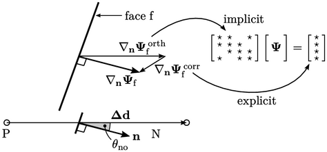
3.8 Surface normal gradient
The surface normal gradient  is a part of the
Laplacian discretisation Eq. (3.2
), illustrated in
the figure below.
is a part of the
Laplacian discretisation Eq. (3.2
), illustrated in
the figure below.
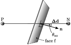
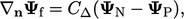
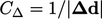
The discretisation of  is built upon a finite
difference of cell values on each side of the face according
to
is built upon a finite
difference of cell values on each side of the face according
to
 |
(3.5) |
 . When this orthogonal scheme
is applied to Eq. (3.2
) to discretise a
Laplacian, it forms coefficients
. When this orthogonal scheme
is applied to Eq. (3.2
) to discretise a
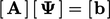
Laplacian, it forms coefficients  of a matrix equation
 since it references cell values of the field
  . For cell
  , the coefficient
for each neighbour cell (
, the coefficient
for each neighbour cell ( ) is
) is 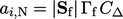 and the diagonal
coefficient is the negative of the sum of neighbour coefficients:
and the diagonal
coefficient is the negative of the sum of neighbour coefficients:
 .
.
Discretisation of  by Eq. (3.5) is most
accurate when the face is orthogonal to
by Eq. (3.5) is most
accurate when the face is orthogonal to
 ,
i.e. the angle
,
i.e. the angle  between
 and
and  is zero. However, if the face is non-orthogonal,
the error associated with Eq. (3.5
) increases with
is zero. However, if the face is non-orthogonal,
the error associated with Eq. (3.5
) increases with  .
.
Non-orthogonal correction
A more accurate discretisation of  at a
non-orthogonal face is formed of the vector sum of the orthogonal
scheme
at a
non-orthogonal face is formed of the vector sum of the orthogonal
scheme  and an explicit
correction
and an explicit
correction  . The latter is calculated from the full gradient
 in
adjacent cells (described in Sec. 3.15
), interpolated to the face
in
adjacent cells (described in Sec. 3.15
), interpolated to the face
 .
.
The correction  is explicit, i.e.
calculated using known values of
is explicit, i.e.
calculated using known values of  , so may need updating
within an iterative sequence to maintain accuracy, as discussed in
Sec. 5.20
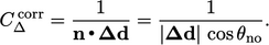
. To ensure that the
iterative sequence converges, the implicit contribution is elevated by replacing
, so may need updating
within an iterative sequence to maintain accuracy, as discussed in
Sec. 5.20
. To ensure that the
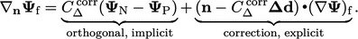
iterative sequence converges, the implicit contribution is elevated by replacing  in the orthogonal
scheme with
in the orthogonal
scheme with
 |
(3.6) |
 scheme combines the implicit and explicit parts by
 |
(3.7) |
 . For
. For  , stability can be
maintained at the expense of accuracy by limiting the magnitude of the
correction
, stability can be
maintained at the expense of accuracy by limiting the magnitude of the
correction  below some fraction of the magnitude of the
orthogonal
below some fraction of the magnitude of the
orthogonal  part.
part.
