
3.9 Advection discretisation
In Sec. 2.8
, we described advection terms
as those of the form  or
or  . The inclusion of velocity
  within the
divergence gives the term particular characteristics that require
special treatment in discretisation.
within the
divergence gives the term particular characteristics that require
special treatment in discretisation.
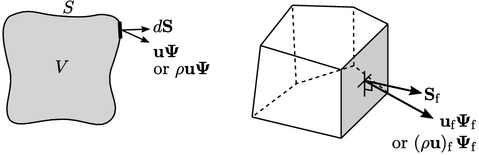
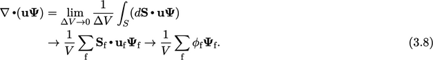
Following the finite volume principles outlined in Sec. 3.1, the discretisation approximates the surface integral by a summation over faces by
The discretisation requires calculation of the
volumetric flux  (see Sec. 2.3
). In the case of
(see Sec. 2.3
). In the case of  included in the
advection term
included in the
advection term  ,
,  is the mass flux
  .
.
In the flux calculation, the interpolation of
 at
cell centres to
at
cell centres to  at faces uses the linear scheme of Sec. 3.7
. Similarly, the
linear scheme is used for the interpolation
at faces uses the linear scheme of Sec. 3.7
. Similarly, the
linear scheme is used for the interpolation  .
.
The critical issue — one of the most important in
CFD numerics — is how to express our advected property  at a face in
terms of values
at a face in
terms of values  in neighbouring cells.
Advection scheme introduction
The advected property  is transported in the
direction of flow velocity
is transported in the
direction of flow velocity  . Interpolation to the face of
  usually
involves the flow direction. In the graphic below a face f is
positioned between two cells. Based on the flow direction, the cells
are labelled upwind ‘U’ and downwind ‘D’.
usually
involves the flow direction. In the graphic below a face f is
positioned between two cells. Based on the flow direction, the cells
are labelled upwind ‘U’ and downwind ‘D’.
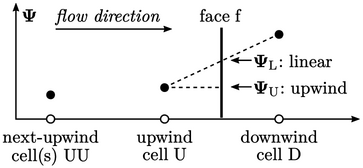
The linear interpolation scheme, 5 described in Sec. 3.7
, does not use
the flow direction but expresses  in terms of adjacent
cells. At first sight, this choice of scheme is logical when
considering accuracy.
However, for advection, the linear scheme tends to generate
unbounded solutions which are unstable.
in terms of adjacent
cells. At first sight, this choice of scheme is logical when
considering accuracy.
However, for advection, the linear scheme tends to generate
unbounded solutions which are unstable.
The upwind
scheme simply represents  by the value in the
upwind cell
by the value in the
upwind cell  . It makes sense from a physical perspective since
particles of fluid in the upwind cell are destined to travel to the
face, transporting property
. It makes sense from a physical perspective since
particles of fluid in the upwind cell are destined to travel to the
face, transporting property  with them.6
While the linear scheme is generally unbounded, the upwind scheme exhibits poor accuracy. In following section we explore the behaviour of upwind before looking at schemes that offer greater accuracy while attempting to maintain boundedness.
