
3.7 Laplacian discretisation
Let us first describe the discretisation of the Laplacian term for diffusion, introduced in Sec. 2.14 .
Following the finite volume principles described in Sec. 3.1, the discretisation approximates the surface integral by a summation over faces by
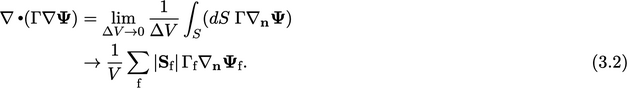
The  in Eq. (3.2
) can be viewed
as the summation over faces of a single cell. Applying the
summation to all cells provides the contribution to coefficients
in Eq. (3.2
) can be viewed
as the summation over faces of a single cell. Applying the
summation to all cells provides the contribution to coefficients
 and
and  of a matrix equation.
The mesh data  and
and  are calculated
according to Sec. 3.3
so the remaining properties to
be determined are:
are calculated
according to Sec. 3.3
so the remaining properties to
be determined are:
- the diffusivity at faces
 ;
; - the surface normal gradient at faces
 .
.
Fields  and
and  are associated with
cells, so numerical schemes are required to evaluate properties at
faces. We will first describe interpolation for
are associated with
cells, so numerical schemes are required to evaluate properties at
faces. We will first describe interpolation for  , for which the linear
scheme is generally used. The surface normal gradient
, for which the linear
scheme is generally used. The surface normal gradient  is discussed
in Sec. 3.8
.
is discussed
in Sec. 3.8
.
Interpolation from cells to faces
Mapping data between different locations is a common practice in numerics. Since the finite volume method is concerned with fluxes at faces, the principal mapping procedure is interpolation from cells to faces. Since other interpolations are much less common, it can be assumed that the term “interpolation” means from cell to face unless stated otherwise.
For irregular polyhedral meshes, interpolation is
generalised by defining a weights field  for each face
according to
for each face
according to
 |
(3.3) |
 is the interpolated face field. The subscripts
  and
and
 indicate values at owner and neighbour cells, respectively.
Linear interpolation
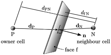
The linear interpolation scheme sets
 according to a linear variation between cells values
  and
and
 .
The weights can then be calculated based on distances from the face
centre to adjacent cell centres, in the direction normal to the
face, by
.
The weights can then be calculated based on distances from the face
centre to adjacent cell centres, in the direction normal to the
face, by
 |
(3.4) |
