Notes on Computational Fluid Dynamics: General Principles

3.15 Gradient discretisation

The discretisation of a gradient is exclusively an explicit calculation using current values of . The conservative form of gradient calculation is based on a surface integral.

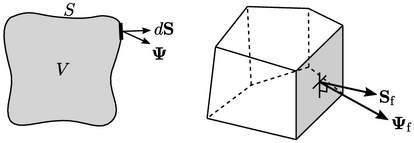
From the gradient definition in Sec. 2.23 , the discretisation is

(3.18)

The face value is generally interpolated from cell values using the linear scheme.

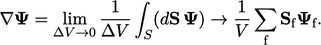
Point linear interpolation

While skewness is generally not a concern for advection discretisation, it deserves greater attention in gradient calculation. For “bad” meshes, e.g. containing elongated tetrahedral cells, the point linear scheme is often adopted to reduce skewness error.

Point linear interpolation uses: the value , calculated using linear interpolation, which corresponds to the “face point” at the intersection of the line connecting cell centres and the face; and, values at each vertex, interpolated from adjacent cells using inverse-distance weighting.

The scheme breaks the polygonal face into triangles and calculates the average value at the 2 vertices and face point for each triangle, area . Point interpolation calculates the face value as the area-weighted average of triangle values, i.e. .

Least squares gradient

A gradient calculation using a least squares finite difference method is sometimes used within the finite volume framework. The method calculates the gradient in a cell which, when used to extrapolate the cell value to centres of all neighbouring cells, minimises the error between extrapolated values and cell values.

For a given cell, a tensor is calculated by summing over faces using the inverse distance weighting 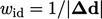, where is the cell centre-centre vector:

(3.19)

The gradient is then evaluated using the inverse of the tensor and values in the neighbour (N) and current (P) cells:

(3.20)