Notes on Computational Fluid Dynamics: General Principles

[chapter contents][previous topic][next topic][index]

3.6 Overview of discretisation

The choice of numerical method determines how coeﬃcients for $\text{[math]}$ and $\text{[math]}$ are calculated and consequently the characteristics of the resulting matrix equation 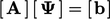$\text{[math]}$ .

The ﬁnite volume method described here is ﬁrmly rooted in the underlying concept of control volumes, described in Sec. 3.1 . It uses integrals over a surface surrounding a volume applied to irregular polyhedral meshes, described in Sec. 3.2 .

The discretisation is described in terms of diﬀerential operators, e.g. $\text{[math]}$ and $\text{[math]}$ , applied to a general ﬁeld $\text{[math]}$ .⁴

$PICT\relax \special {t4ht=$

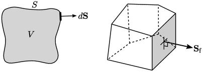
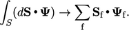
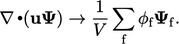
The main concept is that faces within a mesh form closed surfaces surrounding ﬁnite volumes, e.g. a single cell. Any surface integral that represents a derivative, e.g. $\text{[math]}$ , is approximated by a summation over the faces ‘ $\text{[math]}$ ’ that form the surface, i.e.

Z X S(dS ) ! Sf f: f \relax \special {t4ht=

The ﬂux associated with $\text{[math]}$ , i.e. $\text{[math]}$ , must then be calculated. The value $\text{[math]}$ is required at each face, which must be calculated by some method of interpolation of values of $\text{[math]}$ from cells neighbouring the respective face.

Intensive and extensive properties

In this chapter, derivatives and their discretisation are described at a point, e.g. $\text{[math]}$ , e.g. Eq. (3.8 ):

X r (u ) ! 1- f f: V f \relax \special {t4ht=

Calculating a derivative with this expression using the known ﬁeld $\text{[math]}$ simply produces another ﬁeld (with values deﬁned at cell centres, with units of $\text{[math]}$ /time).

The resulting ﬁeld is $\text{[math]}$ , meaning it is independent of the size of the system/geometry. Like other intensive ﬁelds, e.g. $\text{[math]}$ and $\text{[math]}$ themselves, it can be used in further calculations, e.g. within another derivative or added/subtracted from other ﬁelds.

Extensive properties are dependent on the size of the system. For example, the volumetric ﬂux $\text{[math]}$ described in Sec. 3.9 is dependent on the face areas $\text{[math]}$ . Numerical operations involving extensive properties, e.g. addition, subtraction, or mapping to another location, generally produce meaningless data.

While calculations of derivatives yield intensive ﬁelds, matrix equations are constructed in extensive form, with coeﬃcients and source vector scaled by cell volume $\text{[math]}$ . In other words, in the discretisation example above, the multiplication by $\text{[math]}$ would be omitted.

There is no $\text{[math]}$ multiplier in the discretisation of terms which do not involve a surface integral, e.g. time derivative Eq. (3.21 ) and terms in Sec. 3.20 . For those terms, the calculation of matrix coeﬃcients and sources includes a multiplication by $\text{[math]}$ .

⁴consistent with the idea of “Field Operation and Manipulation”, which forms the acronym “FOAM” (later, OpenFOAM) used for the CFD software created by author Henry Weller.

Notes on CFD: General Principles - 3.6 Overview of discretisation