
3.5 Matrix construction
The construction of each matrix equation involves building the matrix and source coefficients from the terms in the equation being solved, with further adjustments for boundary conditions.
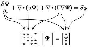
The figure below illustrates the process of
building a matrix equation for a field  from an equation
including advection, diffusion and source
from an equation
including advection, diffusion and source  .
.
 and source
  are calculated for each individual term in the
equation, e.g.
are calculated for each individual term in the
equation, e.g.  ,
,  , etc. using the discretisation methods
described in this chapter.
, etc. using the discretisation methods
described in this chapter.
The overall coefficients are calculated as the sum of coefficients for each term in the the equation. Most terms contribute to both the matrix and source coefficients, although this depends on the choice of discretisation scheme.
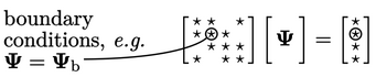
Finally, boundary conditions are incorporated
into the equation through further adjustments to coefficients in
 and
and  as shown below. The adjustments, principally from the
advection and diffusion terms, are applied to coefficients
corresponding to cells at the domain boundary.
as shown below. The adjustments, principally from the
advection and diffusion terms, are applied to coefficients
corresponding to cells at the domain boundary.
Implicit and explicit
The equation for a field  on the previous page
is discretised to form the matrix equation
on the previous page
is discretised to form the matrix equation 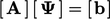 . The discretisation of
a term is implicit when it
contributes to coefficients in
. The discretisation of
a term is implicit when it
contributes to coefficients in  by treating
 as
the solved field
as
the solved field  .
.
Explicit
discretisation calculates coefficients in  only, using current
values of fields. When solving an equation for
only, using current
values of fields. When solving an equation for  , derivatives without
 must be explicit. Terms with
  could be treated
explicitly by using current values of
could be treated
explicitly by using current values of  , but they generally
are not, since explicit solutions are unstable beyond a limiting
time step as described in Sec. 3.17
. A notable exception to this are
the terms discussed in Sec. 3.20
.
, but they generally
are not, since explicit solutions are unstable beyond a limiting
time step as described in Sec. 3.17
. A notable exception to this are
the terms discussed in Sec. 3.20
.
The curl derivative, e.g.  , includes terms in
 and
and  in the decoupled matrix equation for
  . These terms must be
treated explicitly since they do not include
. These terms must be
treated explicitly since they do not include  itself. The situation
for
itself. The situation
for  and
and  is the same, so the curl derivative can be explicit
only.
is the same, so the curl derivative can be explicit
only.
This leaves the following terms which are generally treated implicitly:3
 ;
; ;
; ;
;  , where
  is a scalar.
This chapter details: the discretisation of
these terms, which are generally treated implicitly; and, other
terms such as divergence  and gradient
  which can only be
discretised explicitly within a segregated solution.
which can only be
discretised explicitly within a segregated solution.


