
3.20 Other terms
In an equation for  , there can be terms
other than the time derivative, advection and Laplacian of
, there can be terms
other than the time derivative, advection and Laplacian of
 ,
including:
,
including:
- a linear function
 where
where  is a scalar
coefficient or field;
is a scalar
coefficient or field; - a term without
 , sometimes including
the derivative of another variable, e.g.
, sometimes including
the derivative of another variable, e.g.  .
.
The second example is simply discretised as an explicit gradient term as described in Sec. 3.15 . Derivative terms like this one are described in earlier sections and require no further discussion.
The first example, the  term, requires much
more discussion, particularly relating to the possibility of
implicit discretisation.
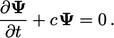
Let us consider the following equation:
term, requires much
more discussion, particularly relating to the possibility of
implicit discretisation.
Let us consider the following equation:
 |
(3.33) |
 is discretised implicitly, then the matrix would contain a zero
diagonal coefficient when
is discretised implicitly, then the matrix would contain a zero
diagonal coefficient when  , making it singular or non-invertible. If this occurs,
 is
not present in the linear equation for the relevant cell, so it
cannot be solved.
is
not present in the linear equation for the relevant cell, so it
cannot be solved.
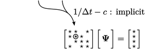
Therefore, such a term must be discretised explicitly
when it has a negative sign (or positive on the right
side of “=”), to ensure the matrix equation is solvable. The nature
of Eq. (3.33
) is that  can only
increase from an initial positive value.
can only
increase from an initial positive value.
Implicit discretisation of linear terms
Let us now consider the equivalent equation with a linear term that has a positive sign, i.e.
 |
(3.34) |
 can only decrease
from an initial positive value but reaches a lower limit at
can only decrease
from an initial positive value but reaches a lower limit at
 .
Like many scalar properties, e.g.
.
Like many scalar properties, e.g.  ,
,  ,
,  , etc.,
  may have a lower
physical bound of 0, which the equation intentionally reflects.
may have a lower
physical bound of 0, which the equation intentionally reflects.
It is important to maintain a physical bound of
 .
Discretisation of Eq. (3.34
) using the Euler time
scheme Eq. (3.21
) gives
.
Discretisation of Eq. (3.34
) using the Euler time
scheme Eq. (3.21
) gives
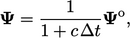 |
(3.35) |
 . An equivalent
explicit discretisation gives
. An equivalent
explicit discretisation gives 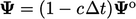 which is only bounded
when
which is only bounded
when  , similar to the
  limit imposed by explicit discretisation of
advection, described in Sec. 3.17
. To avoid this
limit imposed by explicit discretisation of
advection, described in Sec. 3.17
. To avoid this  limit, we apply
implicit discretisation to
terms with a positive sign
on the left side of “=”, where possible.
limit, we apply
implicit discretisation to
terms with a positive sign
on the left side of “=”, where possible.
Even when the term is not linear in  , it can be
implemented as such by “dividing and multiplying by
, it can be
implemented as such by “dividing and multiplying by  ”. For example, the
 turbulence model includes an
  term in the
  equation,
i.e.
equation,
i.e.  , ignoring other
terms. Dividing and multiplying the
, ignoring other
terms. Dividing and multiplying the  term by
  gives
gives
 |
(3.36) |
 which can be discretised implicitly using a
coefficient
which can be discretised implicitly using a
coefficient  .
.
