
7.12 Heat transfer in turbulent flow
The initial focus of turbulence modelling is to capture the effect of mixing on momentum diffusion since it influences the overall flow solution. But other properties are also transported by the turbulent eddying motions, in particular heat.
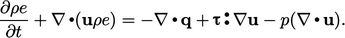
The effects of turbulence on heat transfer can be
described using the following equation for internal energy
 ,
obtained by substituting the material derivative in
Eq. (2.57
) and ignoring
,
obtained by substituting the material derivative in
Eq. (2.57
) and ignoring
 :
:
 |
(7.44) |
 , see Eq. (6.11
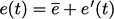
). The ensemble average of the
terms in
, see Eq. (6.11
). The ensemble average of the
terms in  introduces a heat flux
 |
(7.45) |
 , Eq. (6.14
), in momentum. Boussinesq
modelled
, Eq. (6.14
), in momentum. Boussinesq
modelled  by Eq. (6.20
), using the concept of an
eddy viscosity
by Eq. (6.20
), using the concept of an
eddy viscosity  corresponding to turbulent mixing, analogous to
viscosity due to molecular motion according to Newton’s law
Eq. (2.41
).
corresponding to turbulent mixing, analogous to
viscosity due to molecular motion according to Newton’s law
Eq. (2.41
).
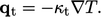
Similarly,  can be modelled using
a turbulent thermal conductivity
can be modelled using
a turbulent thermal conductivity  due to turbulent
mixing, by analogy with Fourier’s law Eq. (2.54
) for conduction due to molecular
interaction
due to turbulent
mixing, by analogy with Fourier’s law Eq. (2.54
) for conduction due to molecular
interaction
 |
(7.46) |
 in Eq. (7.44
) is then
expressed in terms of the combined turbulent mixing and molecular
interaction, using an effective
thermal conductivity
in Eq. (7.44
) is then
expressed in terms of the combined turbulent mixing and molecular
interaction, using an effective
thermal conductivity  , as follows:
 |
(7.47) |
Modelling turbulent heat transfer
Turbulent heat transfer can be incorporated into turbulence models based on eddy-viscosity and Reynolds-averaging, with additional thermal wall functions.
First, the calculation of  by Eq. (7.47) requires
 from the turbulence model. A common approach to calculate
 is
from
is
from  based on an estimate of turbulent Prandtl number
 |
(7.48) |
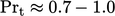 provides a good estimate for many fluids, with
  often chosen as a
default value for CFD calculations. For some more unusual fluids,
e.g. liquid metals,
often chosen as a
default value for CFD calculations. For some more unusual fluids,
e.g. liquid metals,
 .
.
Wall heat flux
The calculation of heat transfer through
boundary walls is an important aspect of a many CFD simulations.
Near walls, the distribution of  tends to mimic
 .
.
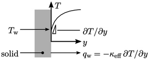
Consequently, the challenges of calculating
wall heat flux  are similar to wall shear stress
  . Cells close to the
wall must be very thin to resolve the viscous sub-layer in
. Cells close to the
wall must be very thin to resolve the viscous sub-layer in
 (when
(when  ).
).
Otherwise, wall functions can be used to adjust
 to
compensate for the under-prediction of
to
compensate for the under-prediction of  as described in
Sec. 7.14
.
as described in
Sec. 7.14
.
