
7.14 Thermal wall functions
Wall functions were introduced in
Sec. 7.5
in order to improve the
calculation of wall shear stress  when cells are too
large near a wall to resolve
when cells are too
large near a wall to resolve  accurately. The same
problem exists with heat flux
accurately. The same
problem exists with heat flux  and an under-predicted
 .
As before, the universal character of the boundary layer can be
exploited, this time to improve the calculation of
.
As before, the universal character of the boundary layer can be
exploited, this time to improve the calculation of  .
.
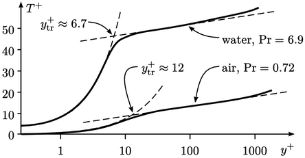
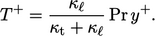
The temperature distribution is characterised
by Eq. (7.51
) for the viscous sub-layer,
and the log law Eq. (7.52
) for the inertial sub-layer.
The transition  for
for  occurs at the intersection of the two
equations, i.e. when
occurs at the intersection of the two
equations, i.e. when
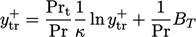 |
(7.57) |
 by
Eq. (7.18
) for the
by
Eq. (7.18
) for the  profile, the
(iterative) solution of Eq. (7.57
) is dependent on
profile, the
(iterative) solution of Eq. (7.57
) is dependent on  and
and  .
.
Using  and Eq. (7.55
) for
and Eq. (7.55
) for  ,
,  for air at
 with
with  . For water under the same conditions,
  and the corresponding
 .
.
A wall function can be derived which adjusts the
turbulent conductivity  , in a similar manner to
  in the standard
wall function in Sec. 7.5
. The model calculates
in the standard
wall function in Sec. 7.5
. The model calculates
 for each patch face based on the near-wall cell
  .
.
No adjustment is made to  when
when  corresponds to the
viscous sub-layer. When
corresponds to the
viscous sub-layer. When  corresponds to the inertial sub-layer,
 is
calculated as
is
calculated as
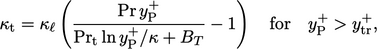 |
(7.58) |
 denotes the laminar thermal conductivity, i.e.
  from
Eq. (2.54
), to distinguish it from
Kármán’s constant
from
Eq. (2.54
), to distinguish it from
Kármán’s constant  . Eq. (7.58
) uses
. Eq. (7.58
) uses  from
Eq. (7.19
), as in the standard
from
Eq. (7.19
), as in the standard
 wall function.
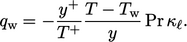
The wall function is derived based on adjusting
 to
improve the numerical calculation of
to
improve the numerical calculation of  by
by
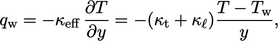 |
(7.59) |
 represents a value close to the wall, e.g. in a near-wall cell. By
comparison, Eq. (7.49
) and Eq. (7.50
) combine to give
represents a value close to the wall, e.g. in a near-wall cell. By
comparison, Eq. (7.49
) and Eq. (7.50
) combine to give
 |
(7.60) |
 is consistent between Eq. (7.59
) and
Eq. (7.60
) when
is consistent between Eq. (7.59
) and
Eq. (7.60
) when
 |
(7.61) |
 according to
Eq. (7.58
).
according to
Eq. (7.58
).
