
6.9 Reynolds-averaged simulation
The computational cost of DNS and, to a lesser extent, LES is too great for most practical CFD, as discussed in Sec. 6.8 . Instead, a Reynolds-averaged simulation (RAS) provides a much more affordable method to calculate turbulence.
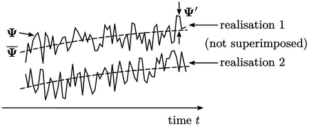
It solves equations for “averaged” field variables to avoid resolving small fluctuations. Rather than consider an average over a time interval, we imagine the same flow repeated several times under nominally the same initial conditions (2 examples below).
Solutions vary due of differences in initial
conditions and the chaotic nature of turbulence. The ensemble average calculates the mean solution  for multiple
realisations of the same flow.
for multiple
realisations of the same flow.
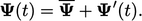
Each field, e.g.  , is decomposed into
the averaged field
, is decomposed into
the averaged field  and field of random fluctuations
  , according to
 |
(6.11) |
 split into
  and
and  as follows:
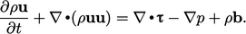 |
(6.12) |
 and that the body force
  is not subject to
turbulent fluctuations. Splitting the remaining fields, i.e.
is not subject to
turbulent fluctuations. Splitting the remaining fields, i.e.  ,
,  and
and  , into
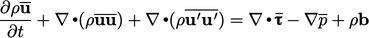
instantaneous and fluctuating components according to
Eq. (6.11
), and taking the ensemble
average of Eq. (6.12
), yields the
following:
, into
instantaneous and fluctuating components according to
Eq. (6.11
), and taking the ensemble
average of Eq. (6.12
), yields the
following:
 |
(6.13) |
 and
and  :
:  ;
;  ;
;  ;
;  . Relations for
averaged derivatives are:
. Relations for
averaged derivatives are:  ;
;  ;
;  .
.
Reynolds stress
The terms for mean quantities in
Eq. (6.13
) are the same as in
Eq. (6.12
). The difference is
that Eq. (6.13
) includes the
additional  term containing fluctuations
  .
.
The argument of this divergence derivative is a tensor known as the Reynolds stress11
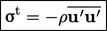 |
(6.14) |
 )
to give
)
to give
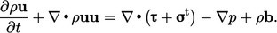 |
(6.15) |
 . Solving this Reynolds-averaged equation is the key to low
cost CFD with turbulence — but it requires a model for the additional unknown
. Solving this Reynolds-averaged equation is the key to low
cost CFD with turbulence — but it requires a model for the additional unknown
 .
.
