
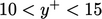
7.7 Turbulence near walls
The characteristic velocity distribution in
turbulent boundary layers in Sec. 7.4
, provided wall
functions expressed as boundary conditions for  in Sec. 7.5
and Sec. 7.6
. Boundary
conditions also need to be specified for turbulence fields at solid
walls.
in Sec. 7.5
and Sec. 7.6
. Boundary
conditions also need to be specified for turbulence fields at solid
walls.
The turbulence generation  influences the
distribution of turbulence fields near a wall. At the wall,
influences the
distribution of turbulence fields near a wall. At the wall,
 .
In the inertial sub-layer,
.
In the inertial sub-layer,  from Eq. (7.5
) with:
from Eq. (7.5
) with:  , obtained by combining
Eq. (6.21
) and Eq. (7.15
); and,
Eq. (6.24
).
, obtained by combining
Eq. (6.21
) and Eq. (7.15
); and,
Eq. (6.24
).
Since  decreases with increasing
  in the inertial
sub-layer,
in the inertial
sub-layer,  passes through a peak within the buffer layer (at
 ).
).
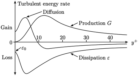
The peak in  causes a similar peak
in
causes a similar peak
in  , shown in the following diagram. To the left of the peak,
turbulent energy is transported back towards the wall by diffusion
, shown in the following diagram. To the left of the peak,
turbulent energy is transported back towards the wall by diffusion
 The profile of dissipation
  results from
 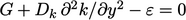 , obtained
from Eq. (7.1
). Very close to the wall
(
, obtained
from Eq. (7.1
). Very close to the wall
( ),
diffusion is predominately molecular, such that it non-zero at the
wall. The dissipation
),
diffusion is predominately molecular, such that it non-zero at the
wall. The dissipation  also has a non-zero value
  at the wall.
Wall functions and turbulence fields
When using a turbulence model, such as the
 model described in Sec. 7.1
, boundary conditions must be
specified for
model described in Sec. 7.1
, boundary conditions must be
specified for  and
and  at solid walls. The distribution of
  ,
non-dimensionalised as
,
non-dimensionalised as  , close to the wall is shown below.
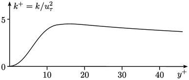
At the wall,  but it rises quickly
to a peak at
but it rises quickly
to a peak at  before levelling off at
  as
as  .
.
With wall functions, the height of the centre of
each near-wall cell should correspond to  within the range
 .
Viewed at that scale, the
.
Viewed at that scale, the  profile appears flat. For
  , there is no such
simple profile shape. These observations lead to the boundary
conditions for
, there is no such
simple profile shape. These observations lead to the boundary
conditions for  and
and  when using wall functions:
- zero
gradient for
 ;
; - calculated
near-wall cell value for
 , according to:
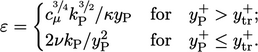 |
(7.26) |
 from the near-wall cell. The expression for
 is
Eq. (7.4
) with Eq. (6.24
). The expression for
is
Eq. (7.4
) with Eq. (6.24
). The expression for
 uses the asymptotic condition
  for
for  in Eq. (7.28
).
in Eq. (7.28
).
