
6.12 Mixing length
By analogy with kinetic theory, the eddy
viscosity  can be expressed in terms of a characteristic speed
 and length
  . Prandtl produced the following model for the mixing
length
. Prandtl produced the following model for the mixing
length  :16
:16
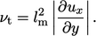 |
(6.21) |
 -direction,
  , carry fluid to the
  plane from a distance
 .
.
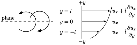
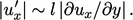
At  , the turbulent fluctuations in the
 -direction,
  , correspond to the range of velocities at
 such that
 |
 , a positive
  at
at  corresponds to a negative
  , and vice versa.
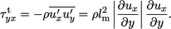
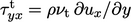
The Reynolds stress
, and vice versa.
The Reynolds stress  can then be constructed by defining a mixing
length
can then be constructed by defining a mixing
length  to replace
  , absorbing the constant of proportionality, to
give
, absorbing the constant of proportionality, to
give
 |
(6.22) |
 , we arrive at
  in Eq. (6.21
).
in Eq. (6.21
).
The mixing length Eq. (6.21) is
only effective as a turbulence model to calculate  when the flow is
simple enough that
when the flow is
simple enough that  can be chosen appropriately.
Such an example is high  , fully-developed flow
through a pipe of radius
, fully-developed flow
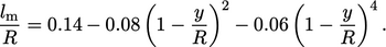
through a pipe of radius  . The mixing length
  , calculated from
measured velocity profiles, follows a polynomial function of
distance
, calculated from
measured velocity profiles, follows a polynomial function of
distance  from the wall, given by17
 |
(6.23) |
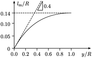
Notably, close to the wall, e.g.  , the mixing length
increases linearly according to
, the mixing length
increases linearly according to
 |
(6.24) |
 is Kármán’s constant.
At the centre of the pipe, 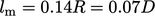 where
where  is pipe diameter.
Estimates of
is pipe diameter.
Estimates of  are commonly cited for other simple examples,
e.g. mixing layer, jet, flat
plate boundary layer, etc.,
where
are commonly cited for other simple examples,
e.g. mixing layer, jet, flat
plate boundary layer, etc.,
where  is the characteristic length of the problem (radius in the
case of a jet).
is the characteristic length of the problem (radius in the
case of a jet).
