
7.8 Resolving the viscous sub-layer
Wall functions were introduced in
Sec. 7.5
to avoid the need for a
large mesh with cells small enough to resolve the boundary layer
into the viscous sub-layer. They provide a reasonable prediction of
 using the log law for the velocity distribution in the inertial
sub-layer.
using the log law for the velocity distribution in the inertial
sub-layer.
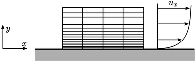
A CFD simulation may alternatively use a mesh
with sufficiently thin cells to resolve the flow through the viscous
sub-layer, e.g. with
near-wall cell centre height corresponding to  = 1, for a more
accurate prediction of
= 1, for a more
accurate prediction of  . If so, the turbulence model must then be
able to function reliably in viscous flow regions.
. If so, the turbulence model must then be
able to function reliably in viscous flow regions.
Such models are usually described as “low
Reynolds number”. The expression does not
refer to the  of the flow based on the characteristic scales of the
problem, e.g. axial mean
flow speed and diameter for a pipe. Instead it is a “turbulence”
Reynolds number
of the flow based on the characteristic scales of the
problem, e.g. axial mean
flow speed and diameter for a pipe. Instead it is a “turbulence”
Reynolds number  based on the scales of speed
  and size
  of turbulent
eddies and can be defined as
of turbulent
eddies and can be defined as
 |
(7.27) |
 . Since
 represents fluctuations,
  . Combining these expressions into a
Reynolds number yields Eq. (7.27
).
. Combining these expressions into a
Reynolds number yields Eq. (7.27
).
Asymptotic consistency
Low- turbulence models pay attention to the
behaviour of fluctuating velocities, e.g.
turbulence models pay attention to the
behaviour of fluctuating velocities, e.g.  ,
,  , in the limit that
 at
the solid boundary.
at
the solid boundary.
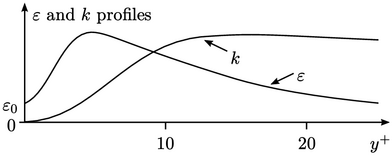
They aim to capture the shape the profiles of
 and
and
 as
they approach
as
they approach  . Let
. Let  and
and  define the directions tangential and normal
to the wall respectively. Profiles in the fluctuating velocities can
be expressed by polynomials in
define the directions tangential and normal
to the wall respectively. Profiles in the fluctuating velocities can
be expressed by polynomials in  , i.e.
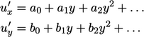 |
 , etc. are functions
of space and time. The no slip condition implies
, etc. are functions
of space and time. The no slip condition implies  , so
, so  to the lowest
order in
to the lowest
order in  . For
. For  , it is
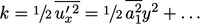
  since, at the wall,
  and by continuity
 .
.
The turbulent properties are, to the lowest order
in  , as follows.

It follows that models achieve asymptotic consistency when
 |
(7.28) |
 .
.
