
7.5 Wall functions
CFD simulations may be used to calculate the
forces on solid bodies exerted by the fluid, e.g. in aerodynamics. The wall shear
stress is then calculated according to 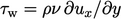 . With turbulent
boundary layers, the
. With turbulent
boundary layers, the  calculation requires cells with very small
lengths normal to the wall to be accurate. The resulting mesh is
inevitably large, which carries a high computational cost. The
problem for CFD is how to calculate
calculation requires cells with very small
lengths normal to the wall to be accurate. The resulting mesh is
inevitably large, which carries a high computational cost. The
problem for CFD is how to calculate  with sufficient
accuracy, but at an affordable cost.
with sufficient
accuracy, but at an affordable cost.
Wall
functions provide a solution to this problem by exploiting
the universal character of the velocity distribution described in
Sec. 7.4
. They use the
law of the wall Eq. (7.13
) as a model to provide a
reasonable prediction of  from a relatively inaccurate
  calculation at
the wall.
calculation at
the wall.
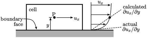
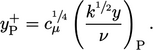
Wall functions use the near-wall cell centre height
 ,
i.e. the distance to the
wall from the centre P of each near-wall cell. Typically when using
wall functions,
,
i.e. the distance to the
wall from the centre P of each near-wall cell. Typically when using
wall functions,  should correspond to a
  within the typical
range of applicability of the log law Eq. (7.13
), i.e.
within the typical
range of applicability of the log law Eq. (7.13
), i.e. 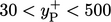 .
.
With such a mesh, the calculated  is then
significantly lower than its true value. Wall function models
compensate for the resulting error in the prediction of
is then
significantly lower than its true value. Wall function models
compensate for the resulting error in the prediction of
 by
increasing viscosity at the wall. The increase is applied to
by
increasing viscosity at the wall. The increase is applied to
 at
the wall patch faces, which would otherwise be
at
the wall patch faces, which would otherwise be  , corresponding to
 .
.
Standard wall function
The standard wall function for a “smooth”
wall calculates  for each patch face based on the near-wall
 .
No adjustment is made to
.
No adjustment is made to  when
when  corresponds to the
viscous sub-layer. When
corresponds to the
viscous sub-layer. When  corresponds to the inertial sub-layer,
 is
calculated by
is
calculated by
 |
(7.17) |
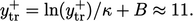
 ) that determines whether
  lies within the
inertial sub-layer corresponds to
lies within the
inertial sub-layer corresponds to  at the intersection of
Eq. (7.11
) and Eq. (7.13
), calculated iteratively as
at the intersection of
Eq. (7.11
) and Eq. (7.13
), calculated iteratively as
 |
(7.18) |
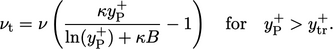
 is
calculated in each near-wall cell according to:
is
calculated in each near-wall cell according to:
 |
(7.19) |
 and Eq. (7.16
). The subscript
and Eq. (7.16
). The subscript
 denotes all properties are evaluated at P.
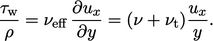
The wall function Eq. (7.17)
is derived from the notion that  is calculated
numerically (assuming a stationary wall) by:
is calculated
numerically (assuming a stationary wall) by:
 |
(7.20) |
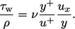 |
(7.21) |
 ,
which combines with Eq. (7.13
) to yield Eq. (7.17).
,
which combines with Eq. (7.13
) to yield Eq. (7.17).
