7.4 Turbulent boundary layers
At solid walls, the tangential flow speed
 increases rapidly across a thin boundary layer, as discussed in
Sec. 6.4
. At high
increases rapidly across a thin boundary layer, as discussed in
Sec. 6.4
. At high  , the velocity
profile has a universal character shown below.
, the velocity
profile has a universal character shown below.
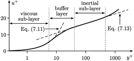
The profile compares measured data in
terms of a dimensionless velocity  and distance to the
wall
and distance to the
wall  , given by

|
(7.9) |
Both parameters in Eq. (
7.9
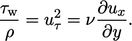
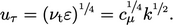
) are based on a
friction velocity 
which is related to
the wall shear stress

by

|
(7.10) |
At the wall

. Close to the wall,

is suppressed,
creating a region where flow is laminar

, known as the
viscous sub-layer . The profile in this
region is described by the relation

|
(7.11) |
Turbulence becomes significant through the
buffer layer which describes the
region

. Van Driest provides a model for the increase in mixing
length through this region, by

|
(7.12) |
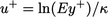
Finally, in the
inertial
sub-layer
for

, flow is turbulent and the velocity profile is described by
the
logarithmic law of the
wall, often abbreviated to simply the
log law, according to
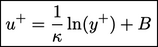
|
(7.13) |
The equation includes Kármán’s constant

and constant

.
For a smooth wall,

– 5.5 is commonly used. Both
Eq. (
7.11
) and Eq. (
7.13) can
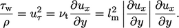
be derived assuming a constant shear stress across the profile,
equating to

at the wall. In the viscous sub-layer, the shear
stress is laminar, so
|
(7.14) |
This equation integrates with a zero constant of integration to
give

, from which Eq. (
7.11
) is derived. In the inertial
sub-layer, the shear stress is turbulent (laminar is negligible),
so
|
(7.15) |
Assuming

gives

, which integrates to yield Eq. (
7.13). In
the inertial sub-layer,

as described in Eq. (
7.5
), which combines with
Eq. (
7.15
) and Eq. (
6.31
) to give
|
(7.16) |