Notes on Computational Fluid Dynamics: General Principles

[chapter contents][previous topic][next topic][index]

7.1 The k-epsilon turbulence model

The $k$ model (k-epsilon) was the ﬁrst turbulence model to be widely adopted for a variety of ﬂows in CFD.² It is one of a family of two equation models which solve two transport equations, one usually for $\text{[math]}$ and one for another variable, often a dissipation rate. These models are the industry standard for CFD.

The $k$ model combines the transport equations for $\text{[math]}$ and $\text{[math]}$ , Eq. (6.28 ) and Eq. (6.32 ) respectively, which are reproduced below assuming $\text{[math]}$ = constant and replacing material derivatives in conservative form as in Eq. (2.26 ).

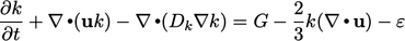(7.1)

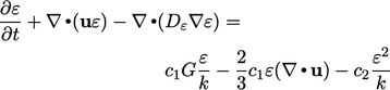(7.2)

The standard model coeﬃcients are

(7.3)

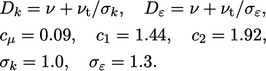The choice of coeﬃcients in Eq. (7.3 ) originates from a large series of validation simulations of free shear ﬂows.³

The model can be deployed in a steady ﬂow solution, setting the local time derivatives to zero, e.g. $\text{[math]}$ . It can also form part of a transient solution to capture unsteady features such as vortex shedding.

The model uses a momentum equation in ensemble-averaged form, e.g. Eq. (6.26 ), using $\text{[math]}$ calculated from updated $\text{[math]}$ and $\text{[math]}$ according to Eq. (6.27 ).

The model equations are added to the end of the main loop in the steady and transient algorithms from Sec. 5.12 or Sec. 5.21 , respectively. The ﬁgure below shows the additions to the transient algorithm, starting from the momentum corrector step.

$PICT\relax \special {t4ht=$

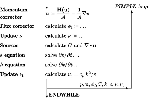
Following the momentum and ﬂux correctors, $\text{[math]}$ can be updated, e.g. for non-Newtonian models where $\text{[math]}$ . $\text{[math]}$ and $\text{[math]}$ are calculated and stored for source terms in both the $\text{[math]}$ and $\text{[math]}$ equations. Those equations are then solved, followed by an update to $\text{[math]}$ , and subsequently $\text{[math]}$ .

²William Jones and Brian Launder, The prediction of laminarization with a two-equation model of turbulence, 1972.

³Brian Launder, Alan Morse, Wolfgang Rodi and Brian Spalding, Prediction of free shear ﬂows — A comparison of the performance of six turbulence models, NASA Conference on Free Shear Flows, Langley, 1972.

Notes on CFD: General Principles - 7.1 The k-epsilon turbulence model