
3.22 Bounded advection discretisation
Sec. 2.9
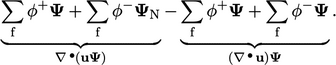
described the conservation
and boundedness qualities of the advective derivatives  and
and
 ,
respectively. According to Eq. (2.31
), the terms are
equivalent when
,
respectively. According to Eq. (2.31
), the terms are
equivalent when  , i.e. when
mass conservation Eq. (2.8
) is satisfied in the case when
, i.e. when
mass conservation Eq. (2.8
) is satisfied in the case when
 constant.
During computation of an incompressible flow,
numerical error can be significant, in particularly at the beginning
of a steady-state calculation. The governing equations are not
satisfied, including mass conservation, so  .
.
Discretisation of an advection term of the form
 as
described in Sec. 3.9
can cause
unboundedness in
as
described in Sec. 3.9
can cause
unboundedness in  . If
. If  has a physical bound that is violated, the
solution rapidly becomes unstable.
has a physical bound that is violated, the
solution rapidly becomes unstable.
The addition of the  term ensures
boundedness while
term ensures
boundedness while  , at the expense of conservation. Once
 ,
the solution is both bounded and conservative.
,
the solution is both bounded and conservative.
 |
(3.43) |
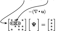
 , so contributes
 to
the diagonal coefficients of the matrix. If
to
the diagonal coefficients of the matrix. If  is positive, we might
expect a singular matrix, as discussed in Sec. 3.20
. However, the decrease to
the diagonal coefficient is matched by an increase from the
discretisation of
is positive, we might
expect a singular matrix, as discussed in Sec. 3.20
. However, the decrease to
the diagonal coefficient is matched by an increase from the
discretisation of  . If that term uses the upwind scheme, the
discretisation can be split into a contribution from positive
outgoing fluxes
. If that term uses the upwind scheme, the
discretisation can be split into a contribution from positive
outgoing fluxes  and negative incoming fluxes
  . In extensive form
(i.e. scaled by
. In extensive form
(i.e. scaled by
 ,
see Sec. 3.24
), using values in the
cell of interest
,
see Sec. 3.24
), using values in the
cell of interest  and neighbouring cells
  , the terms are
 |
 terms cancel, leaving negative coefficients for neighbouring
cells (since
terms cancel, leaving negative coefficients for neighbouring
cells (since  is negative). The diagonal coefficient is then equal to
the sum of magnitude of those neighbour cell coefficients, resulting
in an invertible matrix.
is negative). The diagonal coefficient is then equal to
the sum of magnitude of those neighbour cell coefficients, resulting
in an invertible matrix.
Capturing physics
Boundedness and conservation can be compromised
when a term in an equation does not capture the physics of the
problem. An example from flame speed combustion modelling uses a
parameter  which represents the fraction of the unburnt fuel
mixture.
which represents the fraction of the unburnt fuel
mixture.
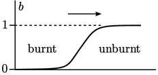
The equation for  includes the source
term
includes the source
term  , where
  is a calculated flame speed. Its inclusion could cause
the solution of
is a calculated flame speed. Its inclusion could cause
the solution of  to fall below its lower bound of 0.
Multiplying and dividing by 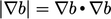 changes the term to
 ,
where
,
where  and unit vector
  . In this form, the term represents the
non-conservative advection of
. In this form, the term represents the
non-conservative advection of  by a flame velocity
 moving in the direction
  , which captures the physical nature of
combustion. Boundedness can then be maintained by a suitable choice
of advection scheme.
, which captures the physical nature of
combustion. Boundedness can then be maintained by a suitable choice
of advection scheme.
