
3.21 Terms which change sign
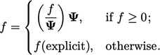
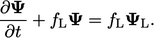
An equation may include a function  which can
return a value which is positive or negative, e.g.
which can
return a value which is positive or negative, e.g.
 |
(3.37) |
 and ensure the solution exceeds the lower bound
of 0 when
and ensure the solution exceeds the lower bound
of 0 when  . The discretisation of
  is therefore treated
implicitly or explicitly within each cell based on
is therefore treated
implicitly or explicitly within each cell based on
 |
(3.38) |
Maintaining lower and upper bounds
The solution variable  could have a physical
bound at any low value
could have a physical
bound at any low value  and/or high value
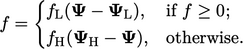
  . We can treat the
function
. We can treat the
function  in Eq. (3.37
) as follows to
maintain boundedness:
in Eq. (3.37
) as follows to
maintain boundedness:
 |
(3.39) |
 and
and  are calculated using the current values of
 .
.
If we examine the situation with  ,
Eq. (3.37
) would be
discretised as
,
Eq. (3.37
) would be
discretised as
 |
(3.40) |
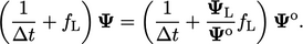
 implicitly alongside the Euler time scheme,
Eq. (3.40
) becomes:
implicitly alongside the Euler time scheme,
Eq. (3.40
) becomes:
 |
(3.41) |
 decreases when
  , but cannot fall below
the
, but cannot fall below
the  bound within a solution step. In the limit that
 ,
the solution for
,
the solution for  no longer decreases.
An equivalent analysis shows Eq. (3.40
) maintains
boundedness for the upper bound  . In that case, note
that
. In that case, note
that  is negative so the term in
  can still be treated
implicitly.
can still be treated
implicitly.
Fields bounded by 0 and 1
Many properties are expressed as a fraction, e.g. concentration of a chemical species, so are bounded by 0 and 1. When that happens, Eq. (3.39 ) simplifies to
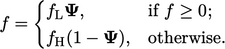 |
(3.42) |
 and
and 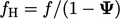 are calculated using the current values of
 .
.
It is particularly important to maintain
boundedness of a field with 0-1 bounds when it is used to calculate
another property which has a physical bound. For example, in a
system of  fluid phases, fluid
  can be calculated by
  from phase fractions
 and densities
  .
.
A small amount of unboundedness in  , in the phase
with highest
, in the phase
with highest  , causes large unboundedness in
  , e.g. in 2 phases with
  and
and  , the
calculated
, the
calculated  with
with  .
.
