
8.6 Automotive aerodynamics
An example of flow around a road vehicle was
used to discuss some boundary conditions in Chapter 4
and to illustrate
the cost of simulating turbulence in Sec. 6.8
. An
aerodynamics simulation was
undertaken to capture the air flow around the vehicle, described by
a CAD model. The aim was to calculate the
drag coefficient at a speed of 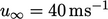 .
.
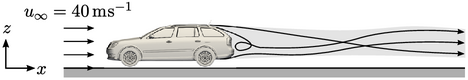
A mesh of 20 million cells was generated, with
the vehicle facing a freestream flow velocity  . The vehicle and
ground formed solid boundaries, with far-field boundaries positioned
. The vehicle and
ground formed solid boundaries, with far-field boundaries positioned
 upstream and
  downstream of the vehicle.
Along the elevated sections of the far-field
boundary, the cell length was  , reducing to
 towards the vehicle by splitting within specified regions.
Additional cell layers along the vehicle surface resulted in a
near-wall cell height of
towards the vehicle by splitting within specified regions.
Additional cell layers along the vehicle surface resulted in a
near-wall cell height of  .
.
The simulation used the steady-state algorithm in
Sec. 5.12
, with an incompressible fluid
with uniform  .
.
The freestream boundary conditions from
Sec. 4.16
were applied to  and
and
 at
the far-field boundaries, with reference values
at
the far-field boundaries, with reference values  ,
,  and
and  . The condition
 was a applied at solid boundaries, with
  applied to the vehicle
and
applied to the vehicle
and  on the ground to emulate their relative motion.
Turbulence was modelled using the  SST model
described in Sec. 7.11
. Turbulence levels
of
SST model
described in Sec. 7.11
. Turbulence levels
of  and
and  were applied at the freestream boundaries and the standard
wall function from Sec. 7.5
was applied at the
vehicle and ground.
were applied at the freestream boundaries and the standard
wall function from Sec. 7.5
was applied at the
vehicle and ground.
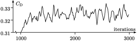
The simulation ran for 3000 iterations using
numerical schemes recommended in Sec. 3.23
. The drag coefficient
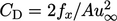 was
calculated from the projected frontal area
was
calculated from the projected frontal area  and the
  -component
 of
the force
of
the force  on the vehicle using Eq. (8.1
).
on the vehicle using Eq. (8.1
).
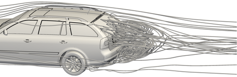
The flow in the wake of the vehicle is naturally
unsteady, which prevents convergence to a steady-state solution.
Beyond 1500 iterations, however, the solution oscillates around an
estimated mean  .
.
