5.12 Steady-state solution
The equations in Sec. 5.10
are combined
using algorithms that couple the solutions for  and
and  . One algorithm is
SIMPLE (Semi-Implicit Method for Pressure-Linked
Equations)3, which is presented here with a modern
interpretation.
. One algorithm is
SIMPLE (Semi-Implicit Method for Pressure-Linked
Equations)3, which is presented here with a modern
interpretation.
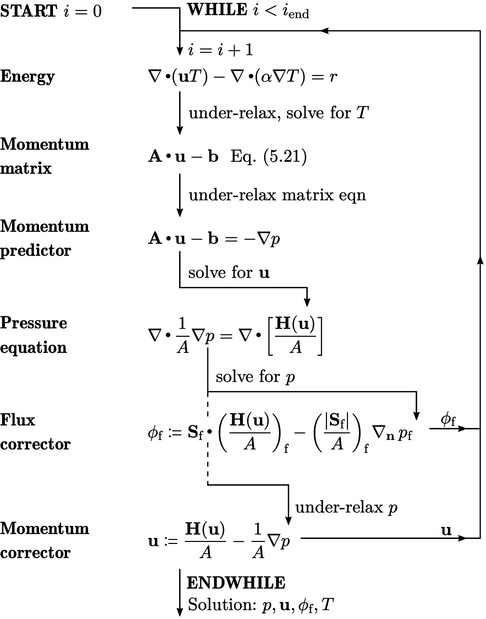
The SIMPLE algorithm is generally used to produce steady flow solutions in CFD. These solutions are directly applicable for flows that reach a steady state, i.e. when flow variables stop changing in time. They can also provide approximate solutions to flows that are moderately unsteady, usually at a lower cost than a more exact transient solution.
An example of the algorithm is shown for the
system of equations presented in Sec. 5.9
. The time derivative
( )
terms are omitted due to the steady-state assumption.
)
terms are omitted due to the steady-state assumption.
The algorithm involves an iterative sequence with
steps,  . It begins by constructing a matrix equation for energy
which is under-relaxed by a factor
. It begins by constructing a matrix equation for energy
which is under-relaxed by a factor  . The equation is
solved for
. The equation is
solved for  , which is used to update
  according to an
equation of state. A matrix equation is then constructed using all
the terms from the momentum equation excluding
according to an
equation of state. A matrix equation is then constructed using all
the terms from the momentum equation excluding  , i.e.
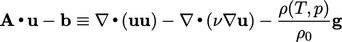 |
(5.21) |
 before equating
with
before equating
with  and solving for
  (the momentum predictor).
 and
and  are then evaluated from
  (the momentum matrix), as described on
page 351.
They are used to form the pressure equation,
which is solved for
(the momentum matrix), as described on
page 351.
They are used to form the pressure equation,
which is solved for  .
.
The new pressure  is used to correct the
flux
is used to correct the
flux  so that it obeys mass conservation better (the flux corrector). It is then under-relaxed by a factor
 before correcting
  before the next solution step begins (the
momentum corrector).
before the next solution step begins (the
momentum corrector).