
8.7 Nonuniform inlet velocity
At an inlet boundary, the velocity is usually
specified by a fixed value condition  , as discussed in
Sec. 4.3
. In many CFD
applications, the flow at an inlet boundary is described by a single
speed which is applied to all faces assuming
, as discussed in
Sec. 4.3
. In many CFD
applications, the flow at an inlet boundary is described by a single
speed which is applied to all faces assuming  is uniform across the
boundary.
is uniform across the
boundary.
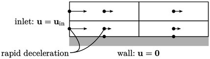
This creates an anomaly where the inlet
boundary meets a wall. In the vicinity of the two boundaries, the
flow decelerates from  at an inlet face to a value in the adjacent
cell close to the no-slip condition
at an inlet face to a value in the adjacent
cell close to the no-slip condition  applied at the wall.
There is inevitably a high “spike” in pressure
and shear stress within the cell in order to decelerate the flow so
rapidly. As the length of the cell (in the flow direction) is
reduced, the deceleration and associated pressure  increases such
that
increases such
that  in the limit that cell volume
  .
.
The solution tends to converge more slowly with the pressure spike, and can be unstable. Furthermore, the spike in shear stress can generate high levels of turbulence which can cause flow separation where the inlet and wall meet.
The uniform condition does not reflect the flow behaviour upstream of the inlet. For example, assuming the wall extends upstream, a boundary layer would have developed at the inlet; or if the wall begins at the inlet, the flow would stagnate at its leading edge.
This is a good example of the axiom that
numerical methods do not respond well to any modelling which is
unphysical. The problems can be avoided by specifying a nonuniform
 which represents the upstream flow better.
Some fields of engineering use established
theories to describe the inlet  , e.g. wind engineering uses a profile of
 based on an atmospheric boundary layer along the earth’s surface.
More generally, a nonuniform  can be specified which
tends to
can be specified which
tends to  at wall boundaries. Profiles can be described by
 where:
  is the normalised velocity and
  is normalised distance
to the nearest wall boundary; and,
is normalised distance
to the nearest wall boundary; and,  and
and  denote the maximum
 and
and  values.
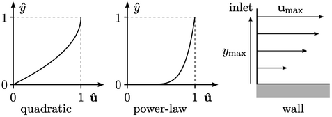
It is logical to specify  using established
profiles for boundary layers as a reasonable estimate for the
upstream conditions. A quadratic function
using established
profiles for boundary layers as a reasonable estimate for the
upstream conditions. A quadratic function  represents a developed boundary layer for
laminar flow, matching the analytical profiles for flow in a pipe or
between flat parallel plates, i.e. Poiseuille’s law.
represents a developed boundary layer for
laminar flow, matching the analytical profiles for flow in a pipe or
between flat parallel plates, i.e. Poiseuille’s law.
Alternatively, a power law function  represents a
developed turbulent boundary layer quite well. Prandtl used
represents a
developed turbulent boundary layer quite well. Prandtl used
 —
his one-seventh power
law3 — to reproduce data for flow in a pipe, but any
suitable exponent
—
his one-seventh power
law3 — to reproduce data for flow in a pipe, but any
suitable exponent  can be used in practice.
