Notes on Computational Fluid Dynamics: General Principles

3.10 Upwind scheme

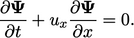
The upwind scheme represents the face value by the value in the cell upwind of the face. The advantage of upwind is that it can guarantee boundedness of a field . We can demonstrate this point by revisiting the 1D Eq. (2.32 ) in Sec. 2.9 :

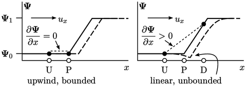
In the graphic above, we track the translation of a profile of by equating changes in in time to the local gradient . If we apply upwind to calculate the change at point P, the gradient and no change in is correctly calculated (left).

However, linear differencing between upwind and downwind values results in , so predicts a decrease in the value at P (right). The solution produces a solution with , so is unbounded.

Boundedness of the conservative form of advection is only guaranteed when , as discussed in Sec. 2.9 . In 1D, the conservative form moves inside the derivative . That gradient is only zero with upwind when is uniform, i.e. the 1D equivalent to .

Diffusion of upwind

The upwind scheme is highly diffusive which can result in poor accuracy. Its diffusive nature can be explained by considering the following Taylor’s series expansion:

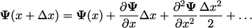(3.9)

In our 1D example, the upwind scheme calculates using and at locations U and P, separated by distance . Relating the upwind calculation to Eq. (3.9 ) gives

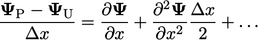(3.10)

In other words, the upwind discretisation represents but also the second derivative (and higher derivatives). is equivalent to a Laplacian, described in Sec. 2.14 , which diffuses with a diffusivity proportional to .

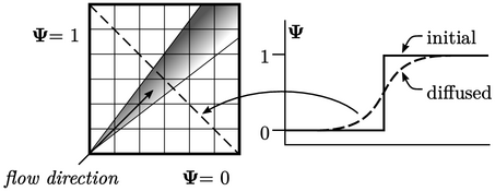
The upwind scheme is particularly diffusive when the flow direction is not aligned with the cells of a mesh. In the 2D box of cells above, is advected at a angle, beginning with an abrupt step change from  = 1 and  = 0 between the left and lower boundaries. The step rapidly diffuses along the direction of travel as shown in graph (right) and shaded area (left).