5.21 The PIMPLE algorithm
The  -
- coupling algorithms in Sec. 5.12
and Sec. 5.19
can be combined into an algorithm
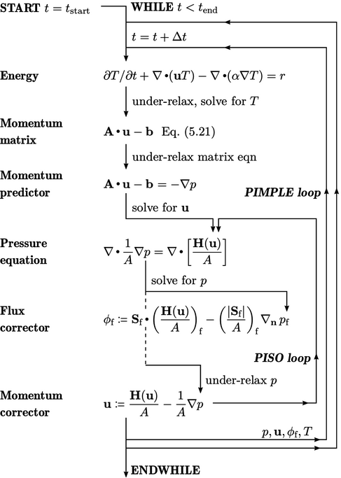
known as PIMPLE. PIMPLE merges the controls of PISO and SIMPLE
(hence the merged acronym), in particular the iterative loops and
under-relaxation.
coupling algorithms in Sec. 5.12
and Sec. 5.19
can be combined into an algorithm
known as PIMPLE. PIMPLE merges the controls of PISO and SIMPLE
(hence the merged acronym), in particular the iterative loops and
under-relaxation.
All controls are optional; the standard transient
algorithm is replicated by deactivating both the under-relaxation
and the PIMPLE loop. By including the PIMPLE loop, equations are
solved using variables updated within the time step. Accuracy is
improved in particular due to the update of matrix coefficients from
the contribution of  to advection.
For transient simulations, temporal accuracy can
be maintained at a higher  (
( ) using a second order time scheme
(Sec. 3.18
) combined with
iterations of the PIMPLE loop. Similarly, the PIMPLE loop can
update explicit source terms, e.g. in energy or momentum, to improve
accuracy.
) using a second order time scheme
(Sec. 3.18
) combined with
iterations of the PIMPLE loop. Similarly, the PIMPLE loop can
update explicit source terms, e.g. in energy or momentum, to improve
accuracy.
Pseudo-transient solution
PIMPLE can be configured to produce a steady flow
solution quickly by a pseudo-transient simulation. These
simulations are not intended to capture realistic transient
behaviour so can run at  with some under-relaxation if necessary.
The simulations can be accelerated to a steady
state using local time
stepping (LTS). LTS recognises that
 is
limited by the maximum
is
limited by the maximum  associated with the cell with small
 and/or high
  . It uses a field of
  corresponding to the
 limit in each cell to
accelerate the transient solution. While using a
limit in each cell to
accelerate the transient solution. While using a  field makes the
transient solution invalid, it is acceptable at steady state when
field makes the
transient solution invalid, it is acceptable at steady state when
 .
.