
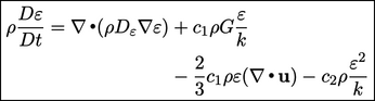
6.14 Turbulent dissipation rate
A complete model for  is still required to
solve the ensemble-averaged momentum equation, e.g. Eq. (6.26
). The discussion in
Sec. 6.11
indicates
is still required to
solve the ensemble-averaged momentum equation, e.g. Eq. (6.26
). The discussion in
Sec. 6.11
indicates  is the product
of
is the product
of  and
and  , requiring two models to represent each scale. Since
 ,
,
 can represent the speed scale, modelled by Eq. (6.28
).
can represent the speed scale, modelled by Eq. (6.28
).
The turbulent dissipation rate  matches the rate of
transfer of kinetic energy down the energy cascade
matches the rate of
transfer of kinetic energy down the energy cascade  , as discussed in
Sec. 6.6
. This applies to all
turbulent scales including the larger mixing length scales, so
, as discussed in
Sec. 6.6
. This applies to all
turbulent scales including the larger mixing length scales, so
 . Substituting
  and
and  expressions into
  yields turbulent
viscosity
yields turbulent
viscosity
 |
(6.31) |
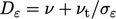
 is a constant. From empirical data,
  , except within the
viscous and buffer layers close to a wall, see Sec. 7.4
.
, except within the
viscous and buffer layers close to a wall, see Sec. 7.4
.
Transport of turbulent dissipation rate
A model is now required for  , both to calculate
 by
Eq. (6.31
) and to provide the
remaining unknown in Eq. (6.28
). The model can be provided
by a transport equation for
by
Eq. (6.31
) and to provide the
remaining unknown in Eq. (6.28
). The model can be provided
by a transport equation for 
 |
(6.32) |
 is the combined
molecular and turbulent diffusion with an adjustable coefficient
is the combined
molecular and turbulent diffusion with an adjustable coefficient
 ,
usually set to 1.3. The remaining coefficients
,
usually set to 1.3. The remaining coefficients  and
and  are tuned to
capture the behaviour of a range of flows.
are tuned to
capture the behaviour of a range of flows.
The  -equation,
Eq. (6.32
), can be derived in terms
of statistical properties, replacing high-order terms in
-equation,
Eq. (6.32
), can be derived in terms
of statistical properties, replacing high-order terms in
 by
models with coefficients
by
models with coefficients  ,
,  .18
.18
Alternatively, it can be obtained by multiplying
the principal variable,  or
or  , in each term of Eq. (6.28
) by
, in each term of Eq. (6.28
) by  and introducing
coefficients
and introducing
coefficients  ,
,  and
and  .
.
The  term in Eq. (6.32)
causes
term in Eq. (6.32)
causes  to increase with
  . This is logical since the generated
turbulence moves down the energy cascade, so ultimately affects the
rate of dissipation.
. This is logical since the generated
turbulence moves down the energy cascade, so ultimately affects the
rate of dissipation.
The  term is justified by considering the
free decay of
turbulence. If the fluid stops moving (
term is justified by considering the
free decay of
turbulence. If the fluid stops moving ( ) and turbulence is no
longer generated (
) and turbulence is no
longer generated ( ), then (assuming constant
  and ignoring diffusion)
Eq. (6.28
) and Eq. (6.32)
reduce to
and ignoring diffusion)
Eq. (6.28
) and Eq. (6.32)
reduce to
 |
(6.33) |
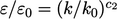 where
the “0” subscript indicates initial values.
where
the “0” subscript indicates initial values.
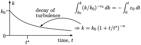
Further integration yields a decay in
 over time to the power
 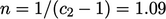 and a timescale
  , which is a
reasonable approximation to real behaviour.
, which is a
reasonable approximation to real behaviour.
