
5.22 Solving for energy
Examples with energy conservation in this
chapter assume  is constant to produce the transport equation for
 in
Eq. (2.65
). When
in
Eq. (2.65
). When
 cannot be assumed to be constant, it is common to solve an equation
for internal energy
cannot be assumed to be constant, it is common to solve an equation
for internal energy  instead, e.g. Eq. (2.60
) with the
material derivative replaced using Eq. (2.14
)
instead, e.g. Eq. (2.60
) with the
material derivative replaced using Eq. (2.14
)
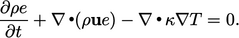 |
(5.39) |
 ,
from which
,
from which  can be solved. The challenge is that the diffusion
term
can be solved. The challenge is that the diffusion
term  is not expressed in terms of
  , so is discretised
explicitly, which adversely affects convergence.
, so is discretised
explicitly, which adversely affects convergence.
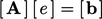
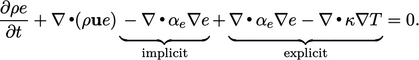
To improve convergence, an implicit term is
introduced which is similar in form and scale to the problem term.
For energy Eq. (5.39
), we
use  , where the diffusivity
  is calculated from the
 function of
  .
.
The extra term is both “added and subtracted” in
implicit and explicit form. This has the effect of increasing the
contributions to matrix coefficients, while cancelling out a large
part of the explicit contribution from  , as illustrated
below
, as illustrated
below
 |
 from
from
 from thermodynamic relationships, e.g. Eq. (2.62
). The equation for
from thermodynamic relationships, e.g. Eq. (2.62
). The equation for
 is
then solved, and the subsequent solution for
is
then solved, and the subsequent solution for  is converted back to
 .
.
If  is expressed as a polynomial function of
 ,
Eq. (2.64
), then
,
Eq. (2.64
), then  is converted to
 using the analytical integral of Eq. (2.62
)
using the analytical integral of Eq. (2.62
)
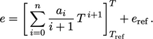 |
(5.40) |
From temperature to energy
The conversion from  to
to  is more complex
because
is more complex
because  cannot be made the subject of Eq. (5.40).
Instead, it can be “inverted” using an iterative scheme such as the
Newton-Raphson method,8
which for this problem is:
cannot be made the subject of Eq. (5.40).
Instead, it can be “inverted” using an iterative scheme such as the
Newton-Raphson method,8
which for this problem is:
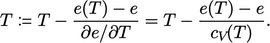 |
(5.41) |
 is
updated from the current
is
updated from the current  using the evaluated
  and
and  polynomials,
Eq. (5.40
) and Eq. (2.64
), respectively. One
iteration is often sufficient for the error
polynomials,
Eq. (5.40
) and Eq. (2.64
), respectively. One
iteration is often sufficient for the error  to fall within a
prescribed tolerance, but further iterations of Eq. (5.41)
can be applied if necessary.
to fall within a
prescribed tolerance, but further iterations of Eq. (5.41)
can be applied if necessary.
Boundary conditions
The boundary conditions for the energy equation
are generally specified in terms of  . But since they must
be applied to the variable being solved, they must be reposed in
terms of
. But since they must
be applied to the variable being solved, they must be reposed in
terms of  . A fixed value condition
  is converted to an
equivalent condition
is converted to an
equivalent condition  , e.g.
by Eq. (5.40
). A fixed gradient
condition
, e.g.
by Eq. (5.40
). A fixed gradient
condition  for
for  is converted to a fixed gradient
  for
for  by
by
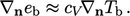 |
(5.42) |
