
7.9 Low-Re k-epsilon models
There are many low- turbulence models for
CFD simulations where the cells near the solid walls are sufficiently
thin to resolve the flow through the viscous sub-layer.
turbulence models for
CFD simulations where the cells near the solid walls are sufficiently
thin to resolve the flow through the viscous sub-layer.
Among them are several low-
 models based on
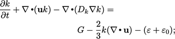
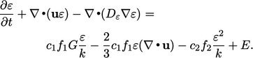
Eq. (7.1
) and Eq. (7.2
) with additional corrections
models based on
Eq. (7.1
) and Eq. (7.2
) with additional corrections
 ,
,
 ,
,
 and
and
 :
:
 |
(7.29) |
 |
(7.30) |
 also includes a correction
  :
:
 |
(7.31) |
 publication.12 They proposed
functions for
publication.12 They proposed
functions for  ,
,  ,
,  ,
,  and
and  , as well as the coefficients
  ,
,  and
and  .
.
Launder and
Sharma subsequently presented13
the model with a modified  function and the more established
coefficients listed in Eq. (7.3
).
function and the more established
coefficients listed in Eq. (7.3
).
The resulting model became known as the
Launder-Sharma  model.14 It is arguably the most popular
low-
model.14 It is arguably the most popular
low- model today.
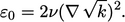
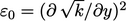
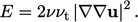
The first notable modification to the standard
 model is
  (sometimes denoted “
 ”) in
Eq. (7.29
). It is the dissipation
rate at the wall (
”) in
Eq. (7.29
). It is the dissipation
rate at the wall ( ), see figure, Sec. 7.7
, calculated by
), see figure, Sec. 7.7
, calculated by
 |
(7.32) |
 in the boundary layer which is
consistent with Eq. (7.28
). The benefit of
redefining the dissipation rate as
in the boundary layer which is
consistent with Eq. (7.28
). The benefit of
redefining the dissipation rate as  is that the boundary
conditions at a wall for the Launder-Sharma model are the same for
is that the boundary
conditions at a wall for the Launder-Sharma model are the same for
 and
and
 :
:
- fixed
value
 ;
; - fixed
value
 .
.
The next significant modification is the
 function
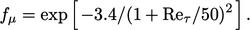 |
(7.33) |
 so decreases
 through the buffer and viscous sub-layer to the wall, consistent
with the decrease in
through the buffer and viscous sub-layer to the wall, consistent
with the decrease in  according to the van Driest model
Eq. (7.12
).
according to the van Driest model
Eq. (7.12
).
The extra term  in Eq. (7.30)
is a follows, designed so that
in Eq. (7.30)
is a follows, designed so that  matches its recognised
peak value within the buffer layer:
matches its recognised
peak value within the buffer layer:
 |
(7.34) |
 and
and  provide damping of the production and dissipation
terms close to the wall in Eq. (7.30
). The standard functions are
provide damping of the production and dissipation
terms close to the wall in Eq. (7.30
). The standard functions are  (i.e. no damping), and
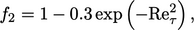 |
(7.35) |
 at the wall.

