3.3 Finite volume mesh
The finite volume numerical method is closely associated with the concept of surface and volume integrals used in Chapter 2 . Below, we extract the main geometric elements from the figures used for the conservation laws.
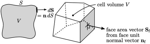
The integrals use volumes  and area vectors
 .
The numerical method uses equivalent discrete quantities for cells
and faces:
.
The numerical method uses equivalent discrete quantities for cells
and faces:
 ;
; ,
, ;
; .
.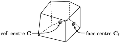
The finite volume method relates discrete values
of fields, e.g. pressure, to
cells and faces within the mesh. For many calculations data must to
be assigned to point locations, in particular the cell centre (more
specifically centroid) and face centre
  .
.
Calculating mesh data
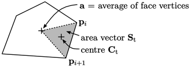
To calculate  , each polygonal face is
decomposed into triangles using an apex point
, each polygonal face is
decomposed into triangles using an apex point  . The area vector
 and
centre
and
centre  are then calculated for each triangle according to
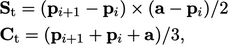
 ” is the cross product, Eq. (2.70
). The sum of area vectors
gives
” is the cross product, Eq. (2.70
). The sum of area vectors
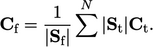
gives  and
and  is the area weighted sum of triangle centres over
 triangles, calculated by
 |
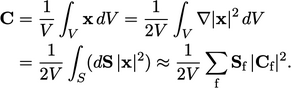
 can be
calculated from
can be
calculated from  and
and  by Gauss’s theorem, using
  to describe position
and noting
to describe position
and noting  . The surface integral (
 ) becomes a sum over
cell faces
) becomes a sum over
cell faces  , replacing discrete values
  and
and  for
for  and
and  respectively as
follows:
respectively as
follows:
 |
 , by
, by