Notes on Computational Fluid Dynamics: General Principles

5.14 Descent methods

The Gauss-Seidel method, introduced in Sec. 5.2 , provides convergent solutions for many problems in CFD. It is most effective when a modest reduction in residual is required, e.g. as part of a steady-state solution described in Sec. 5.12 .

When the Gauss-Seidel method requires a lot of sweeps (e.g. over 10) to converge to a suitable tolerance, alternative methods may be more efficient. Descent methods provide alternative matrix solvers that are often used in CFD.

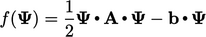
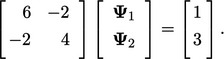
Descent methods represent the equations which are being solved as a minimisation problem. It is demonstrated below using a matrix equation of the form with 2 values

(5.27)

The minimisation presents the equation in quadratic form; in matrix notation, it is a scalar function of the form

(5.28)

The quadratic form of Eq. (5.27 ), is:

(5.29)

The gradient of is:

(5.30)

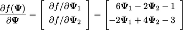
Critically, , i.e. the negative of the residual vector Eq. (5.10 ), as verified by the model example.

Equating the gradient to zero, 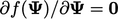, corresponds to a minimum in the quadratic function. At the same time, it is the solution to . The method is therefore concerned with finding the minimum of the quadratic form efficiently.

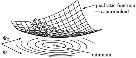
For this method to work, the quadratic form must have a minimum, which requires that is symmetric and positive-definite. A positive-definite matrix is hard to visualise, but for a 2-value function it ensures the quadratic function is a paraboloid.

Diagonal dominance is the convergence condition for the Gauss-Seidel method, discussed in Sec. 5.3 . Importantly, a symmetric matrix that is diagonally dominant, and has positive diagonal coefficients, is also positive-definite.

Matrix operations

The ‘’ operation between two single-column matrices, e.g. , in Eq. (5.28 ) is represented in other texts using matrix notation by a transpose . For the example in Eq. (5.27 ), it is:

(5.31)