Notes on Computational Fluid Dynamics: General Principles

5.2 Gauss-Seidel method

Finite volume numerics generally uses iterative methods to solve each matrix equation. These methods calculate approximate solutions for , which become more accurate with successive iterative solutions.

Iterative methods are preferred because they are more efficient than direct methods, which solve a matrix equation exactly. Gaussian elimination, which is the numerical basis for direct solution methods, has a computational cost . This is prohibitive for many sizes of mesh in finite volume CFD.

Gauss-Seidel¹ is a simple, iterative method which is generally effective for solving transport equations such as the example in Sec. 5.1 . The method is illustrated by a sample equation

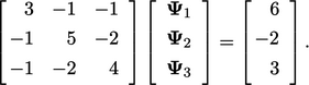(5.2)

The equations can be rewritten by: a) multiplying the off-diagonal coefficients by ; b) subtracting the result from the right hand side (r.h.s.); c) and, dividing by the diagonal coefficient. i.e.:

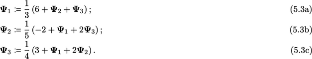
Starting with, 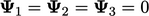, new values of are calculated by Eq. (5.3a ), Eq. (5.3b) and Eq. (5.3c ) in sequence, where the notation “” denotes “ is assigned the value of ”.

The first solution of Eq. (5.3a) is . The updated is substituted in Eq. (5.3b), whose solution is . Both updated values are substituted in Eq. (5.3c ) to give .

The process is then repeated and through successive sweeps over the equations the solution converges as shown below.

The error is 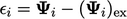, i.e. the difference between the approximate and exact values , and . After 9 sweeps for all variables, i.e. within  0.2% of the exact solution.

In summary, the Gauss-Seidel method is the following sequence of calculations for 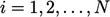, repeated until convergence:

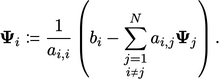(5.4)

The Gauss-Seidel method, applied to sparse matrices, has a computational cost , making it practical for simulations with large meshes that often occur in finite volume CFD.

Convergence of the method, and convergence measures for iterative methods in general, are discussed in the following sections.

---

---