Notes on Computational Fluid Dynamics: General Principles

5.13 Steady-state convergence

The absence of a time derivative from an equation written in steady-state form reduces the diagonal dominance, and hence convergence, of the resulting matrix equation, as discussed in Sec. 5.5 . Under-relaxation is therefore applied to , and to promote convergence in the algorithm in Sec. 5.12 .

The and fields use equation under-relaxation with factors and , respectively. A value of 0.7 is commonly applied, decreasing to 0.5 for less convergent cases (and sometimes to 0.3 in compressible flow cases, beyond the scope of this book).

Under-relaxation of is more subtle. The flux corrector requires that is not under-relaxed to ensure obeys mass conservation better. For the momentum corrector, field under-relaxation is subsequently applied to with a factor . To find an optimal for the momentum corrector, we examine

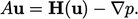(5.22)

This explicit momentum equation contains diagonal coefficients and an off-diagonal contribution 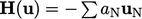from neighbour cell coefficients and associated velocities .

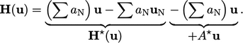
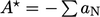Convergence is compromised by the explicit nature of . It can be more implicit by “adding and subtracting” , where coefficients are applied to in the “owner” cells:

(5.23)

Combining Eq. (5.22 ) and Eq. (5.23) gives

(5.24)

which attempts to make Eq. (5.22 ) more implicit in .⁴ The pressure equation derived from Eq. (5.24) is:

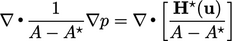(5.25)

This corresponds to under-relaxation of Eq. (5.19 ) by , where 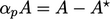. A momentum matrix with coefficients is approximately diagonally equal since there is no time derivative. Since represents the diagonal coefficients under-relaxed by , . Relating the expressions for and gives the optimal under-relaxation factor for for convergence as

(5.26)

leading to the popular choice of and .

Residual control

The algorithm in Sec. 5.12 uses a fixed number of solution steps . In practice, must be chosen to be large enough to reach an acceptable level of convergence. Once convergence is reached, the simulation should stop to avoid unnecessary computing cost.

A common stopping criterion applies a residual level for each equation, below which the equation is deemed to be converged. When all equations satisfy their respective residual controls, the simulation then stops.

Convergence can also be determined by monitoring any suitable metric, including objective measurements from the simulation, e.g. a force coefficient. When the metric no longer changes significantly over subsequent steps, the simulation is stopped.

---

---