
6.4 Boundary layers
Boundary layers4 are
regions of fluid formed along solid boundaries in which the velocity
 varies: from zero at the boundary (no-slip condition,
Sec. 4.4
); to a value largely unaffected
by the proximity of the boundary, determined by the flow
conditions.
varies: from zero at the boundary (no-slip condition,
Sec. 4.4
); to a value largely unaffected
by the proximity of the boundary, determined by the flow
conditions.
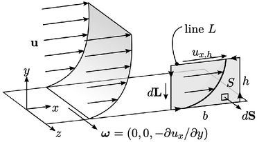
The figure above shows a boundary layer for flow
in the  -direction at speed
  , along a flat solid boundary oriented in the
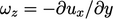
 -normal direction. At the boundary surface, the vorticity
 is
significant.
is
significant.
Vorticity can be shown over a planar section of
the boundary layer of width  and height
 (above, right). Applying Stokes’s theorem, Eq. (2.39
), the integral =
(above, right). Applying Stokes’s theorem, Eq. (2.39
), the integral =
 along the upper line (with zero along the wall and the verticals
sides). The average vorticity over plane area
along the upper line (with zero along the wall and the verticals
sides). The average vorticity over plane area  is therefore
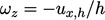 .
.
Boundary layers are the main source of vorticity
for turbulence. Turbulence occurs when instabilities, e.g. induced by roughness of the
boundary surface, cause the vorticity to become chaotic, sustained
by a sufficiently high  .
.
The growth of boundary layers is related to
vorticity transport. For flow over a flat plate, vorticity generated
at the leading edge is advected by the flow, while diffusing away
from the plate.
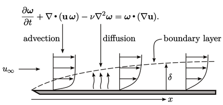
 in time
  , see
Sec. 2.22
. In that time, it is advected
a distance
, see
Sec. 2.22
. In that time, it is advected
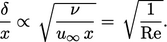
a distance  , where
  is the freestream flow speed. Comparing the
distances over the same
is the freestream flow speed. Comparing the
distances over the same  , the boundary layer thickness is
 |
(6.6) |
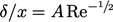 is suitable for laminar boundary layers, with coefficient
 depending on the definition of
  . Data and analysis,
including e.g. the Blasius
solution5,
indicate
. Data and analysis,
including e.g. the Blasius
solution5,
indicate  in the case of the “99% thickness”, i.e. the distance from the wall where
velocity reaches 99% of its asymptotic value.
in the case of the “99% thickness”, i.e. the distance from the wall where
velocity reaches 99% of its asymptotic value.
In turbulent boundary layers, the diffusion
front advances more rapidly due to mixing, see Sec. 6.11
. As a result,
 is
relatively insensitive to
is
relatively insensitive to  , e.g. the analytical solution
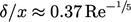 ,
based on a one-seventh (
,
based on a one-seventh ( ) power law for the velocity profile.
