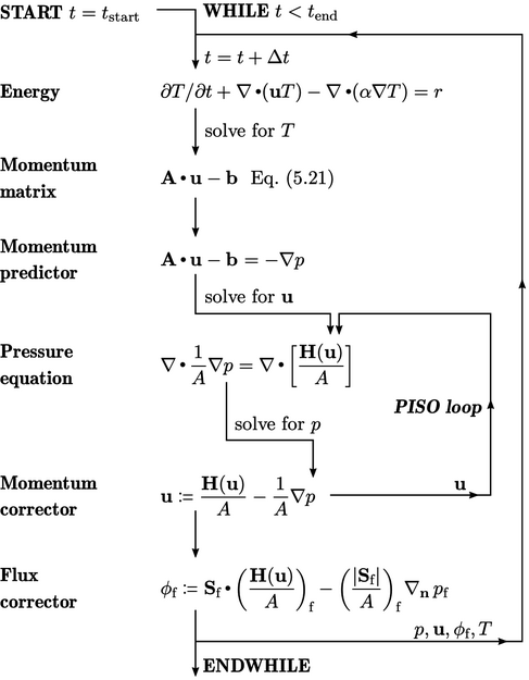
5.19 Transient solution
A modern interpretation of the SIMPLE algorithm
was described in Sec. 5.12
to couple steady solutions for
 and
and  . An equivalent transient solution follows an iterative
sequence in which equations for
. An equivalent transient solution follows an iterative
sequence in which equations for  and
and  are solved over
successive time intervals
are solved over
successive time intervals  , between a start time
  and end time
 .
.
In a transient simulation,  needs to be relatively
small to maintain sufficient accuracy as the solution evolves over
time
needs to be relatively
small to maintain sufficient accuracy as the solution evolves over
time  . The equations do not then generally require
under-relaxation to converge due to the increase of
. The equations do not then generally require
under-relaxation to converge due to the increase of  to the diagonal
coefficients of the matrix from discretisation of the time derivative
to the diagonal
coefficients of the matrix from discretisation of the time derivative
 .
.
A transient simulation could follow the same
sequence as the SIMPLE algorithm on page 359
, but iterating over that sequence
within each time step is costly. A more efficient algorithm solves
the sequence only once per time step but adds an iterative loop
which substitutes  from the momentum corrector into the
  term of the pressure
equation.
term of the pressure
equation.
The pressure equation is then solved a second
time, followed by a second momentum corrector, in the style of the
PISO
algorithm.7 The
addition of this “PISO loop” improves the accuracy of  ,
,  and
and
 within each time step. The improved
  becomes
  in the next
time iteration, which critically increases the accuracy of the time
derivative
in the next
time iteration, which critically increases the accuracy of the time
derivative  in the momentum equation.
Without any iteration over the entire system of
equations, the advection terms are discretised using  from the
previous time step. This “lagging” of
from the
previous time step. This “lagging” of  does not compromise
accuracy significantly, if
does not compromise
accuracy significantly, if  is sufficiently small, e.g. corresponding to
 .
.
A further iteration of the PISO loop can be introduced to solve a third pressure equation and momentum corrector, in particular as part of an update to non-orthogonality described in Sec. 5.20 . Increasing the iterations still further is generally not beneficial.