
3.18 Second order time schemes
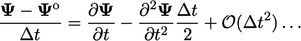
A Taylor’s series
expansion between the current time  and ‘old’ time at
 relates to the Euler implicit scheme by
 |
(3.25) |
 , i.e.
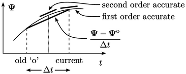
it is first order accurate
in time when the time derivative relates to
, i.e.
it is first order accurate
in time when the time derivative relates to  at the current time, as shown in the
figure below. Despite its low order, the Euler scheme is sufficiently
accurate for many simulations since
at the current time, as shown in the
figure below. Despite its low order, the Euler scheme is sufficiently
accurate for many simulations since  is generally small
when it corresponds to
is generally small
when it corresponds to  .
.
Nevertheless, a second order time scheme may be
required for simulations that demand higher temporal accuracy or to
enable greater computational efficiency by running with larger
 .
.
Backward scheme
In Eq. (3.25
) we can replace
 by
the values
by
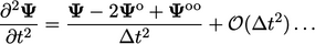
the values  at ‘old-old’ time
  . Subtracting the
expression from Eq. (3.25
) and rearranging terms
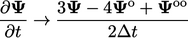
gives the following relation for the second derivative
. Subtracting the
expression from Eq. (3.25
) and rearranging terms
gives the following relation for the second derivative
 |
(3.26) |
 ,
,
 and
and  :
:
 |
(3.27) |
Crank-Nicolson scheme
An implicit solution
expresses the terms in an equation, e.g. advection, Laplacian, at the
current time. The
Crank-Nicolson
method,13
expresses the terms at the midpoint between the current and old
times, to make the Euler time scheme second order accurate.
Denoting discretised terms except the time derivative by
 ,
the Crank-Nicolson method solves
,
the Crank-Nicolson method solves
![@ 1 1 ---- + --[A jb ] + --[A jb ]o o = 0; @t Euler 2 2 \relax \special {t4ht=](img/index1359x.png) |
(3.28) |
 is calculated using
old time values
is calculated using
old time values  .
.
A modern version of the scheme replaces the two
 factors by
  and
and  , introducing the ‘offset coefficient’
  , where
 corresponds to Euler implicit and
  is Crank-Nicolson
Eq. (3.28
). If
is Crank-Nicolson
Eq. (3.28
). If  is discretised
implicitly (as normal), the
Crank-Nicolson scheme can be represented as a time derivative
discretised by
is discretised
implicitly (as normal), the
Crank-Nicolson scheme can be represented as a time derivative
discretised by
![@---- -------o o o @t ! (1 + ) t + [A jb] : \relax \special {t4ht=](img/index1369x.png) |
(3.29) |
 is generally used to ensure solution stability.
