
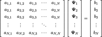
5.1 Structure of matrices
As described in Sec. 3.4
, a matrix equation for
solution variable  contains of a set of coefficients
  where each row
 corresponds to the linear equation for the cell with index
 as
follows:
as
follows:
 |
(5.1) |
Matrix sparsity
Imagine creating a matrix equation for a
transport equation for a scalar field, e.g. Eq. (2.65
) with
zero heat source  .
.
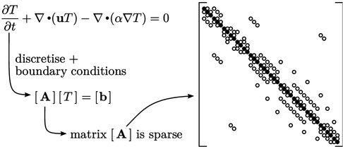
The figure shows a matrix of size  , where
 is
the number of cells. Circles denote non-zero coefficients, which are
filled for the diagonal coefficients (
is
the number of cells. Circles denote non-zero coefficients, which are
filled for the diagonal coefficients ( ). The matrix
 is
sparse, i.e. the majority of the coefficients
is
sparse, i.e. the majority of the coefficients
 are 0 (zero).
The sparsity is due to each cell interacting only with adjacent cells connected through its faces. For example, a 3D mesh of hexahedral cells produces up to 7 coefficients per matrix row, with one diagonal coefficient corresponding to a particular cell and 6 off-diagonal coefficients for the neighbour cells.
Matrix (a)symmetry
A symmetric matrix possesses the same
coefficients across the diagonal, i.e.  . The discretisation of
a Laplacian term, e.g.
. The discretisation of
a Laplacian term, e.g.
 ,
described in Sec. 3.7
, produces
coefficients that are symmetric because the surface normal gradient
Eq. (3.5
) uses the current and
neighbour cell values in equal measure.
,
described in Sec. 3.7
, produces
coefficients that are symmetric because the surface normal gradient
Eq. (3.5
) uses the current and
neighbour cell values in equal measure.
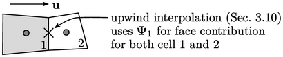
However, the discretisation of an advection term, e.g.  , generally produces
asymmetric coefficients. For
example, if the upwind scheme is applied for flow from cell 1 into
cell 2, then there would a contribution to
, generally produces
asymmetric coefficients. For
example, if the upwind scheme is applied for flow from cell 1 into
cell 2, then there would a contribution to  but not to
 .
.
Matrix size
Parallel simulation allows affordable solution
on huge meshes. For a mesh of size  , the matrix would have
 coefficients, typically with
  that are are non-zero.
For reasons of efficiency, zero coefficients are not stored in the computer’s memory. Instead the storage provides an array of non-zero coefficients and addressing arrays of the corresponding row and column indices for each coefficient.
