3.4 Equation discretisation
Equation discretisation converts partial
differential equations for continuous fields, e.g. pressure  , into sets of linear
equations for discrete
fields.
, into sets of linear
equations for discrete
fields.
The values of the principal fields, e.g.  , are associated with
cells. A field is then represented by an array of values,
, are associated with
cells. A field is then represented by an array of values,
 ,
for cell indices
,
for cell indices 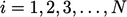 .
.  is the total number of cells.
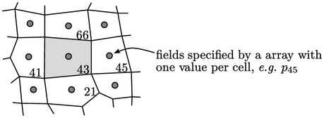
Equation discretisation creates a linear equation for each cell. For cell 43 above, the equation might have the following form:
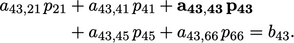
where  and
and  are coefficients corresponding to cell
indices
are coefficients corresponding to cell
indices  ,
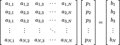
, (diagonal coefficient in bold). The set of linear equations for
all cells can be written as a matrix equation of the form:
(diagonal coefficient in bold). The set of linear equations for
all cells can be written as a matrix equation of the form:
 |
(3.1) |
 where each row
 corresponds to the linear equation for the cell with index
 .
Each row of coefficients are non-zero only for the respective cell
(diagonal
.
Each row of coefficients are non-zero only for the respective cell
(diagonal  ) and near-neighbours. All other coefficients are zero, making
the matrix extremely sparse.
) and near-neighbours. All other coefficients are zero, making
the matrix extremely sparse.
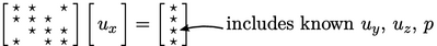
The matrix equation can be represented as
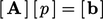 ,
where:
,
where:  are the matrix coefficients;
  are the source
coefficients
are the source
coefficients  ; and,
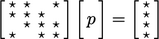
  is the discretised pressure field. It may also be
illustrated as follows, where ‘
is the discretised pressure field. It may also be
illustrated as follows, where ‘ ’ indicates non-zero
coefficients.
’ indicates non-zero
coefficients.
 |
Segregated solution
A CFD simulation generally solves a set of
physical equations, e.g.
for mass, momentum and energy conservation. The finite volume method
traditionally discretises each physical equation separately to form
individual matrix equations for single solution variables,
e.g.  ,
,  ,
,  , rather than creating
a single matrix equation that represents all the physical
equations.
, rather than creating
a single matrix equation that represents all the physical
equations.
The segregated matrix equations are solved
one variable at a time, e.g. solving for  ,
,  and
and  in separate steps.
Where the solution variable is a vector or tensor, e.g.
in separate steps.
Where the solution variable is a vector or tensor, e.g.  , it is decoupled into
individual matrix equations for each component, e.g.
, it is decoupled into
individual matrix equations for each component, e.g.  ,
,  ,
,  .
.
The matrix equations are solved in an
iterative sequence, in which the equation for one variable,
e.g.  , incorporates current
values of other variables, e.g.
, incorporates current
values of other variables, e.g.  ,
,  and
and  , into the source
vector, as shown below.
, into the source
vector, as shown below.