Notes on Computational Fluid Dynamics: General Principles

[chapter contents][previous topic][next topic][index]

5.11 Boundary ﬂuxes

The equations in Sec. 5.10 are used to compute the velocity $\text{[math]}$ , ﬂux $\text{[math]}$ and pressure $\text{[math]}$ based on conservation of mass and momentum. At boundaries, the ﬂux corrector Eq. (5.18 ) must calculate $\text{[math]}$ in a manner consistent with $\text{[math]}$ and $\text{[math]}$ and their respective boundary conditions.

For example, at an impermeable stationary wall the calculated ﬂux must be $\text{[math]}$ , consistent with the no-slip condition $\text{[math]}$ . At boundary faces, $\text{[math]}$ and $\text{[math]}$ must be compatible to evaluate the correct $\text{[math]}$ according to Eq. (5.18 ).

$PICT\relax \special {t4ht=$

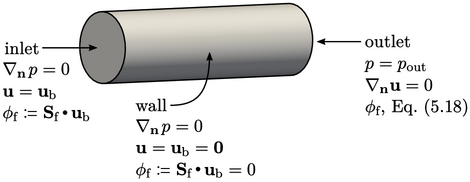
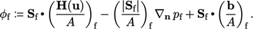
The ﬁgure shows the fundamental boundary conditions from Sec. 4.3 and corresponding ﬂux evaluations. At the inlet and wall boundaries, $\text{[math]}$ is directly assigned from the boundary velocity $\text{[math]}$ by $\text{[math]}$ within the ﬂux corrector Eq. (5.18 ).

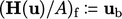In the absence of body forces, the $\text{[math]}$ boundary condition is commonly applied, as discussed in Sec. 4.4 . The ﬂux $\text{[math]}$ is then equivalent to assigning $\text{[math]}$ in Eq. (5.18 ).

At the outlet, $\text{[math]}$ is not prescribed since $\text{[math]}$ is not a ﬁxed value condition. Instead, $\text{[math]}$ is evaluated from Eq. (5.18 ) using $\text{[math]}$ taken from cells adjacent to the boundary and $\text{[math]}$ calculated on the boundary.

Fluxes with a body force

When a body force $\text{[math]}$ is present in the momentum equation, the gradient condition for $\text{[math]}$ , e.g. at an inlet or wall, in principle becomes $\text{[math]}$ , as discussed in Sec. 4.4 . The precise details of the boundary condition in fact depend on how $\text{[math]}$ is incorporated within the coupling algorithm, discussed below.

$PICT\relax \special {t4ht=$

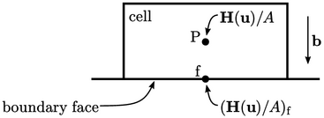
One approach, illustrated by the algorithm in Sec. 5.10 , is to include the body force $\text{[math]}$ within $\text{[math]}$ in Eq. (5.16 ). In that case, the assignment $\text{[math]}$ cannot be valid, so $\text{[math]}$ is adopted instead.

With $\text{[math]}$ established, the $\text{[math]}$ condition is calculated based on the known $\text{[math]}$ by inverting Eq. (5.18 ). This approach causes $\text{[math]}$ to include a contribution from viscous stresses, as in Eq. (4.5 ), which may cause instability.

To avoid this problem, $\text{[math]}$ is omitted from $\text{[math]}$ in Eq. (5.16 ), appearing instead as an extra term in the other equations in Sec. 5.10 , e.g. the ﬂux corrector Eq. (5.18 ) which becomes

ℬ S H(u)- jSfj- r p + S b- : f f A f A f n f f A f \relax \special {t4ht=

(5.20)

Assigning $\text{[math]}$ at boundaries where $\text{[math]}$ is ﬁxed satisﬁes Eq. (5.20 ) when $\text{[math]}$ . This is the condition ignoring viscous stresses described in Sec. 4.4 .

Notes on CFD: General Principles - 5.11 Boundary ﬂuxes