
5.10 Pressure-velocity coupling
The previous section combined equations for
 and
and  , governing momentum and mass conservation, in a sequential
solution.
, governing momentum and mass conservation, in a sequential
solution.
The algorithms used to couple these equations, in
a manner which is convergent, uses the following notation to
describe terms in the momentum equation, e.g. Eq. (2.67
),
excluding 
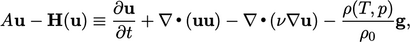 |
(5.16) |
 is a linear term in
  ;
; is a function of
  and other
sources.
and other
sources.
Momentum corrector
A momentum corrector equation is formed by expressing the momentum equation, e.g. Eq. (2.67 ) in terms of the notation of Eq. (5.16 ), and rearranging to give
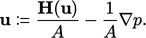 |
(5.17) |
 , based on current
values of
, based on current
values of  and
and  substituted on the r.h.s. In other words,
 and
and  are calculated explicitly.
In the algorithms described in the following
sections,  is chosen to be the extracted diagonal coefficients

 of
the matrix
of
the matrix  corresponding to the momentum terms in
Eq. (5.16
).
corresponding to the momentum terms in
Eq. (5.16
).
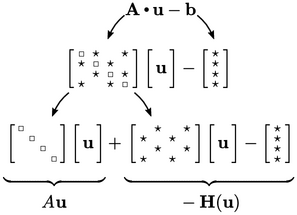
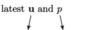
The split between  and
and  is shown above. As
a matrix with diagonal components only,
is shown above. As
a matrix with diagonal components only,  has one value per cell
so can be represented as a scalar field. Setting
has one value per cell
so can be represented as a scalar field. Setting  to be the diagonal
coefficients is a natural choice for implicit treatment of
to be the diagonal
coefficients is a natural choice for implicit treatment of
 within the coupling algorithm.
Flux corrector
A flux
corrector equation follows from Eq. (5.17)
by interpolating  to cell faces and evaluating
  according to
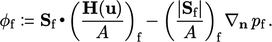 |
(5.18) |
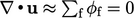
Pressure equation
A pressure
equation is then created by substituting fluxes  from
Eq. (5.18
) into the mass
conservation Eq. (2.46
) in discrete form
from
Eq. (5.18
) into the mass
conservation Eq. (2.46
) in discrete form
 .
The resulting expression is equivalent to a discretised pressure
equation, with coefficients containing
.
The resulting expression is equivalent to a discretised pressure
equation, with coefficients containing  and
and  ,
,
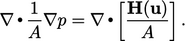 |
(5.19) |
