
3.13 Limiting multiple components
The calculation and application of a limiter is
introduced in Sec. 3.11
for advection of a
single scalar property. The figure below examines when the advected
property is a vector, e.g.
 in
the momentum conservation Eq. (2.47
).
in
the momentum conservation Eq. (2.47
).
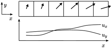
It shows a 2D cut along the  -
- plane through a
selection of cells in a regular mesh with the velocity vector
plane through a
selection of cells in a regular mesh with the velocity vector
 displayed for each cell. When
  is interpolated to
faces along the
is interpolated to
faces along the  -direction using a limited scheme, the simplest
approach is to calculate a limiter for each vector component,
e.g.
-direction using a limited scheme, the simplest
approach is to calculate a limiter for each vector component,
e.g.  , and interpolate the
component with that limiter.
, and interpolate the
component with that limiter.
In the example above, the profiles of  and
and
 in
the
in
the  -direction are quite different, so the calculated limiters
will be different for
-direction are quite different, so the calculated limiters
will be different for  and
and  components at each face. The limiting will
not be invariant under a rotation of the
co-ordinate axes, leading to a different solution depending on the
initial orientation of the geometry with respect to the axes.
components at each face. The limiting will
not be invariant under a rotation of the
co-ordinate axes, leading to a different solution depending on the
initial orientation of the geometry with respect to the axes.
The limiting can be invariant using a single
limiter calculated from the magnitude  , which is applied to
all components of
, which is applied to
all components of  . The strength of the limiting corresponds to an
average across the components, which is usually insufficient for the
component which requires strongest limiting. This can cause
instability.
. The strength of the limiting corresponds to an
average across the components, which is usually insufficient for the
component which requires strongest limiting. This can cause
instability.
Instead, the ‘V’
scheme calculates the limiter based on the ‘worst-case’
direction, i.e. the
direction of steepest gradient in  at the cell face. It
uses the following expression for
at the cell face. It
uses the following expression for  for a vector
 ,
replacing Eq. (3.12
) for a scalar:
,
replacing Eq. (3.12
) for a scalar:
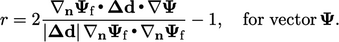 |
(3.17) |
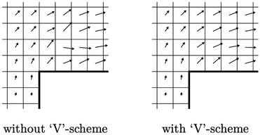
While the V scheme ensures invariance, it also provides greater stability than component limiting. It can remove oscillations in solutions, e.g. in the example above of supersonic flow over a step showing the effect in velocity in the cells adjacent to the step corner.
Multivariate limiting
Multivariate limiting applies the same limiter
for advection discretisation across a set of 2 or more equations.
It works by calculating the limiter  for each solution
variable in the equation set and applying the lowest
for each solution
variable in the equation set and applying the lowest  to all
equations.
to all
equations.
It can be used in order to maintain consistency
in the transport of individual fluid species, such as  ,
,  , e.g. in the propagation of laminar flame
(which is beyond the scope of this book).
, e.g. in the propagation of laminar flame
(which is beyond the scope of this book).
